What you’ll learn

• the one-line structural difference: rules are written, models are derived
• a real contest on the same data: 30 hand-tuned rules (0.7167) vs one default model (0.7667)
• why the 5-point accuracy gap is the least interesting part of that result
• how each approach responds to more data: one improves, one cannot
• why a rule gives you one operating point and a model gives you the whole curve
• when writing the rules is still the correct engineering decision

Intuition

In traditional programming you supply the data and the rules, and the computer produces the answers. In machine learning you supply the data and the answers, and the computer produces the rules.

  flowchart LR
  subgraph TP["Traditional programming"]
    D1["Data"] --> P1["Rules you wrote"]
    P1 --> A1["Answers"]
  end
  subgraph ML["Machine learning"]
    D2["Data"] --> P2["Learning algorithm"]
    A2["Answers (labels)"] --> P2
    P2 --> R2["Rules — the fitted model"]
  end

That inversion is the entire idea, and it sounds almost like a word game until you watch it happen on a problem where the rules are genuinely hard to write.

The contest

Two thousand short messages, half spam and half not. A spam message draws more of its words from a promotional vocabulary — free, winner, prize, click, urgent, offer, cash, limited, guarantee, bonus — and a legitimate message draws more from a work vocabulary. But most words in every message are neutral filler, and roughly a third of the loaded words come from the wrong vocabulary.

Here is one of each:

spam: send report work take week your guarantee guarantee that you will meeting also call about ...
ham : have review here you you deadline here notes report want invoice send for would there and ...

spam: send report work take week your guarantee guarantee that you will meeting also call about ...
ham : have review here you you deadline here notes report want invoice send for would there and ...

You cannot separate those by eye, which is exactly the point. Real spam looks like real mail.

The traditional approach

Write a rule. Flag a message if it contains at least t words from the keyword list. Two knobs: how many keywords, and how many hits it takes to fire. Try every combination — 10 keyword lengths × 3 thresholds = 30 hand-tuned variants.

Watch the failure mode. Adding keywords drives recall up (0.2633 → 0.9833) and precision down (0.6423 → 0.5641), because a longer list fires on more legitimate mail. Raising the threshold pushes back the other way. You are hand-searching a trade-off curve, and the best point you find is 0.7167.

The learned approach

from sklearn.feature_extraction.text import CountVectorizer
from sklearn.naive_bayes import MultinomialNB
 
vec = CountVectorizer()
model = MultinomialNB().fit(vec.fit_transform(X_train), y_train)

from sklearn.feature_extraction.text import CountVectorizer
from sklearn.naive_bayes import MultinomialNB
 
vec = CountVectorizer()
model = MultinomialNB().fit(vec.fit_transform(X_train), y_train)

Two lines. No keyword list, no threshold, no tuning, no domain knowledge. Accuracy 0.7667, precision 0.7614, recall 0.7767.

figureThirty hand-tuned rule variants, none of them enoughmatplotlib

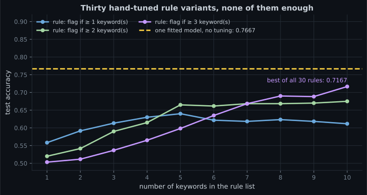
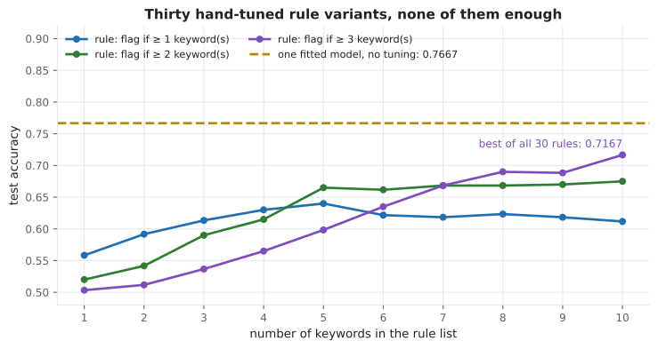
Five points is a real but unspectacular win. It is also, by some distance, the least interesting thing that just happened.

Three differences the accuracy number hides

1. The model found the vocabulary itself

The rule needed a human to sit down and think of ten spam words. The model was handed raw text and discovered 55 distinct tokens, weighting each by how much evidence it carries. It never needed a domain expert, and it would have worked identically on a language nobody in the room speaks.

2. Only one of them improves with data

This is the structural difference, and it is not close.

At 20 examples the rule wins by 16 points. The rule is better than the model, and if you stopped there you would ship the rule.

By 500 examples the model has overtaken it, and the rule’s column never moves — it cannot move, because a rule is a constant. Every new labelled message is free improvement for one approach and inert for the other.

figureOnly one of these two lines responds to more datamatplotlib

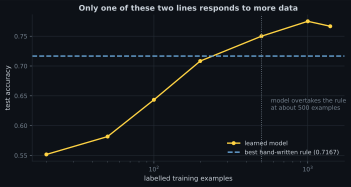
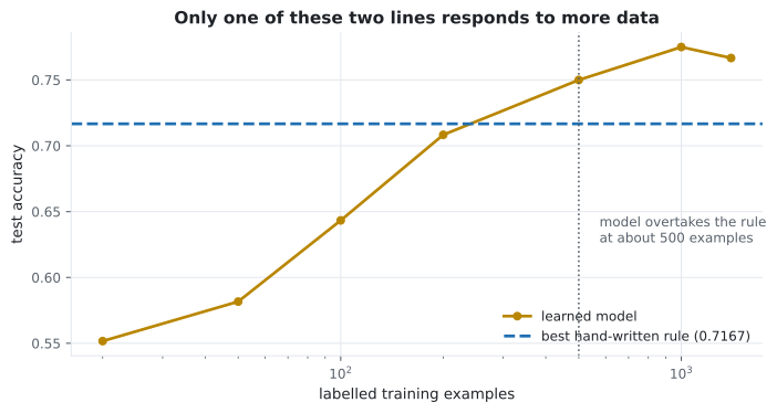
That last detail is worth keeping. The model scores 0.7750 at 1,000 examples and 0.7667 at 1,400. Learning curves wobble; a single dip is not a regression to investigate.

See it move

The rule tree is the honest picture of what maintaining a rule engine feels like after two years. The model’s box never changes size — every new edge case is another row, not another branch.

3. A rule is one operating point; a model is a curve

Every rule variant is a single fixed (precision, recall) pair. Want more recall? Rewrite it and re-measure. The model outputs a probability, so moving the threshold sweeps the entire trade-off without refitting anything.

figureThirty rules give thirty points; one model gives the whole curvematplotlib

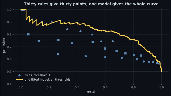
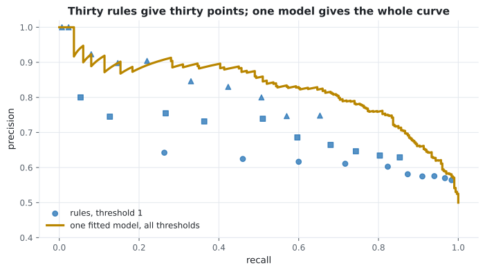
In production this matters more than the headline accuracy. “Legal says we need 95% precision on auto-deletion” is a threshold change with a model, and a rewrite with rules.

What changes in your workflow

The last two rows are where teams get hurt. A rule that breaks throws an exception. A model that breaks returns a plausible number, in the right format, at normal latency, and nothing alerts.

When to write the rules anyway

Machine learning is not a default. Choose it deliberately.

The honest heuristic: if you can write the rule, write the rule. Machine learning earns its complexity when the rules would be numerous, unknown, or moving.

There is also a hybrid answer that is often correct: a small set of hard rules for the cases you know (block this sender, always allow this domain), with a model handling the residue. That is what most real spam filters actually are.

In code

The full contest, reproducible:

import numpy as np
from sklearn.feature_extraction.text import CountVectorizer
from sklearn.metrics import accuracy_score, precision_score, recall_score
from sklearn.model_selection import train_test_split
from sklearn.naive_bayes import MultinomialNB
 
SPAM_WORDS = ["free", "winner", "prize", "click", "urgent",
              "offer", "cash", "limited", "guarantee", "bonus"]
 
def keyword_rule(docs, keywords, threshold):
    """The traditional program: no learning, no data, just logic."""
    kw = set(keywords)
    return np.array([int(sum(w in kw for w in d.split()) >= threshold)
                     for d in docs])
 
X_train, X_test, y_train, y_test = train_test_split(
    docs, labels, test_size=0.3, random_state=0, stratify=labels)
 
# Search all 30 hand-written variants, by brute force, the way a human would.
best = max(
    (accuracy_score(y_test, keyword_rule(X_test, SPAM_WORDS[:k], t)), k, t)
    for k in range(1, 11) for t in (1, 2, 3)
)
print("best rule:", round(best[0], 4), "with", best[1], "keywords, threshold", best[2])
# best rule: 0.7167 with 10 keywords, threshold 3
 
# One fit. No tuning. No keyword list.
vec = CountVectorizer()
model = MultinomialNB().fit(vec.fit_transform(X_train), y_train)
pred = model.predict(vec.transform(X_test))
print("model    :", round(accuracy_score(y_test, pred), 4))     # 0.7667
print("vocabulary:", len(vec.vocabulary_))                      # 55

import numpy as np
from sklearn.feature_extraction.text import CountVectorizer
from sklearn.metrics import accuracy_score, precision_score, recall_score
from sklearn.model_selection import train_test_split
from sklearn.naive_bayes import MultinomialNB
 
SPAM_WORDS = ["free", "winner", "prize", "click", "urgent",
              "offer", "cash", "limited", "guarantee", "bonus"]
 
def keyword_rule(docs, keywords, threshold):
    """The traditional program: no learning, no data, just logic."""
    kw = set(keywords)
    return np.array([int(sum(w in kw for w in d.split()) >= threshold)
                     for d in docs])
 
X_train, X_test, y_train, y_test = train_test_split(
    docs, labels, test_size=0.3, random_state=0, stratify=labels)
 
# Search all 30 hand-written variants, by brute force, the way a human would.
best = max(
    (accuracy_score(y_test, keyword_rule(X_test, SPAM_WORDS[:k], t)), k, t)
    for k in range(1, 11) for t in (1, 2, 3)
)
print("best rule:", round(best[0], 4), "with", best[1], "keywords, threshold", best[2])
# best rule: 0.7167 with 10 keywords, threshold 3
 
# One fit. No tuning. No keyword list.
vec = CountVectorizer()
model = MultinomialNB().fit(vec.fit_transform(X_train), y_train)
pred = model.predict(vec.transform(X_test))
print("model    :", round(accuracy_score(y_test, pred), 4))     # 0.7667
print("vocabulary:", len(vec.vocabulary_))                      # 55

And the part that only the model can do:

proba = model.predict_proba(vec.transform(X_test))[:, 1]
 
for threshold in (0.3, 0.5, 0.7, 0.9):
    flagged = (proba >= threshold).astype(int)
    print(f"threshold {threshold}: "
          f"precision {precision_score(y_test, flagged, zero_division=0):.4f}  "
          f"recall {recall_score(y_test, flagged):.4f}")

proba = model.predict_proba(vec.transform(X_test))[:, 1]
 
for threshold in (0.3, 0.5, 0.7, 0.9):
    flagged = (proba >= threshold).astype(int)
    print(f"threshold {threshold}: "
          f"precision {precision_score(y_test, flagged, zero_division=0):.4f}  "
          f"recall {recall_score(y_test, flagged):.4f}")

No refitting. The model was trained once; the business decision about precision versus recall happens at prediction time, where it belongs.

Pitfalls

Comparing a tuned rule against an untuned model, or vice versa. The comparison above gave the rules 30 attempts and the model one, with defaults. That is deliberately generous to the rules, and it should be — otherwise the result proves nothing.

Concluding “ML wins” from 0.7667 vs 0.7167. Five points on one synthetic corpus is not a law of nature. The durable findings are the shape of the curves: rules are flat in data, models are not; rules are points, models are curves.

Reaching for ML at n=20. The measured table shows the rule beating the model by 16 points there. Small data is rule territory.

Forgetting the model needs labels. The rule needed zero labelled examples. The model needed 1,400. Somebody had to produce those, and that cost is invisible in every accuracy comparison ever published.

Assuming the model is unmaintainable and the rules are not. In practice a rule engine that has accreted 400 exceptions over six years is far harder to reason about than a retrainable model with a held-out score.

Recap

• Traditional programming: data + rules → answers. Machine learning: data + answers → rules.
• On identical data: 30 hand-tuned rules peaked at 0.7167; one default MultinomialNBMultinomialNB fit reached 0.7667.
• The model discovered a 55-token vocabulary with no domain input.
• The rule is flat in data by construction. The model went 0.5517 → 0.7750 and overtook the rule at roughly 500 examples — but lost to it at 20.
• A rule is one (precision, recall) point; a model is the whole curve, selectable at prediction time. Average precision 0.8269.
• If you can write the rule, write the rule.

🧪 Try It Yourself

Exercise 1 – Write the traditional program

Exercise 2 – Search all thirty rule variants

Exercise 3 – Learn the rule instead

Exercise 4 – Which one responds to more data?

Exercise 5 – One model, every operating point

Exercise 6 – Find the size at which the model earns its place

Next

The Machine Learning Roadmap — where the work actually goes, counted line by line in a complete end-to-end pipeline.