Gradients of Vector-Valued Functions

The previous page ended with a $1\times n$ row. This page stacks $m$ of them.

That is genuinely all the new content — and the fact that it is so little is the payoff for §5.2’s row convention. Under the column convention this page would need transposes; under the row convention the gradient of a function with $m$ outputs is just $m$ gradients written one above the other, and the shape rule stays (rows are outputs, columns are inputs) all the way up.

What is new is what the resulting matrix means. Its determinant is a volume magnifier, which is where Chapter 6’s change-of-variables formula comes from. And the chain rule becomes an honest matrix product, which is where backpropagation comes from.

What you’ll learn

• Definition 5.6: the Jacobian of $f:\mathbb{R}^n\to\mathbb{R}^m$ as an $m\times n$ matrix.
• The numerator layout the book uses, its transpose the denominator layout, and how to tell which one a source is using.
• Example 5.9: $\mathrm{d}(\mathbf{A}\mathbf{x})/\mathrm{d}\mathbf{x} = \mathbf{A}$, exactly — the identity every linear layer’s backward pass is.
• The Jacobian determinant as the factor by which areas and volumes scale, verified by counting rather than quoting §4.1.
• Why that is only a local statement for a nonlinear map, measured — and what happens where the determinant vanishes.
• Example 5.10 and 5.11: the chain rule as a matrix product, and the least-squares gradient that Chapter 9 is built on.

Intuition: one row per output

A function with one output has one thing to say about how it changes: a single gradient row. A function with $m$ outputs has $m$ things to say, one per output coordinate, and each is a row.

Stack them and you have a matrix. Row $i$ is “how output $i$ responds to each input”; column $j$ is “how input $j$ affects each output”. Both readings are useful, and they are the two ways to slice the same object.

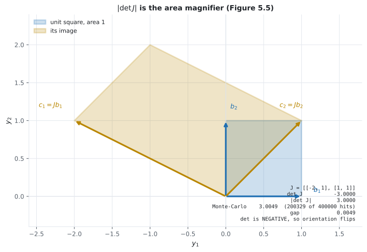
The determinant then answers a question neither row nor column does: how much does the map stretch space? A unit square in the domain lands on a parallelogram in the codomain, and $\lvert\det\mathbf{J}\rvert$ is the ratio of their areas.

diagram Diagram mermaid

  flowchart TD
  F["f: ℝⁿ → ℝᵐ
m outputs, n inputs"]
  F --> ROWS["one gradient ROW per output:
∂fᵢ/∂x = [∂fᵢ/∂x₁ … ∂fᵢ/∂xₙ]"]
  ROWS --> J["Jacobian J ∈ ℝᵐˣⁿ
Def 5.6, Eq 5.58
rows = outputs, cols = inputs"]
  J --> NUM["numerator layout
(the book's choice)"]
  NUM -->|"transpose"| DEN["denominator layout
(also common — check which)"]
  J --> SPECIAL["special cases:
m = 1 → the row of §5.2
n = 1 → a column
f(x) = Ax → J = A exactly"]
  J --> DET["det J: the volume magnifier
Eq 5.58-5.61, Figure 5.5"]
  DET --> CV["Ch 6 §6.7
change of variables"]
  DET --> ZERO["det J = 0: the map folds
— locally not invertible"]
  J --> CHAIN["chain rule as a matrix product
d(f∘g)/dt = (∂f/∂x)(∂x/∂t)"]
  CHAIN --> LS["Example 5.11: ∂L/∂θ = −2eᵀΦ
the gradient Ch 9 runs on"]
  CHAIN --> BP["§5.6 backpropagation"]

The math

The Jacobian

Definition 5.6 — Jacobian

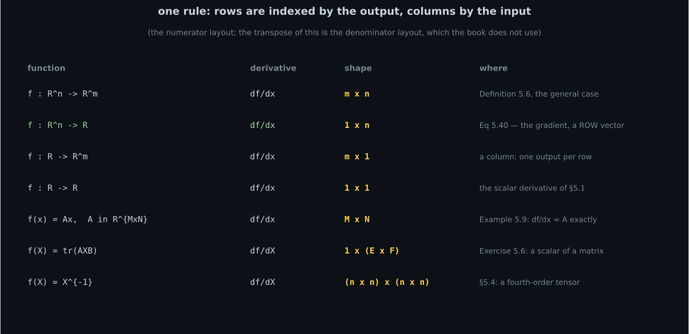
The collection of all first-order partial derivatives of a vector-valued function $f:\mathbb{R}^n\to\mathbb{R}^m$ is called the Jacobian. The Jacobian $\mathbf{J}$ is an $m\times n$ matrix, defined and arranged as

$$\mathbf{J} = \nabla_\mathbf{x}f = \frac{\mathrm{d}f(\mathbf{x})}{\mathrm{d}\mathbf{x}} = \begin{bmatrix}\dfrac{\partial f(\mathbf{x})}{\partial x_1} & \cdots & \dfrac{\partial f(\mathbf{x})}{\partial x_n}\end{bmatrix} = \begin{bmatrix} \dfrac{\partial f_1(\mathbf{x})}{\partial x_1} & \cdots & \dfrac{\partial f_1(\mathbf{x})}{\partial x_n}\\ \vdots & & \vdots\\ \dfrac{\partial f_m(\mathbf{x})}{\partial x_1} & \cdots & \dfrac{\partial f_m(\mathbf{x})}{\partial x_n} \end{bmatrix} \tag{5.58}$$

with $J(i,j) = \partial f_i/\partial x_j$.

As a special case, a function $f:\mathbb{R}^n\to\mathbb{R}^1$ has a Jacobian that is a row vector of dimension $1\times n$ — which is exactly Equation 5.40. §5.2 was not a different construction; it was this one with $m = 1$.

Remark — the layout convention

The book uses the numerator layout: the derivative $\mathrm{d}f/\mathrm{d}\mathbf{x}$ of $f\in\mathbb{R}^m$ with respect to $\mathbf{x}\in\mathbb{R}^n$ is an $m\times n$ matrix, where the elements of $f$ define the rows and the elements of $\mathbf{x}$ define the columns. There also exists the denominator layout, which is the transpose of the numerator layout.

The two differ unless the Jacobian happens to be square, so this is not a convention you can leave unresolved. A quick test on any source: find a Jacobian of a map with different input and output dimensions and read its shape. $\mathbb{R}^3\to\mathbb{R}^4$ gives $4\times3$ in numerator layout and $3\times4$ in denominator layout.

The Jacobian determinant

§4.1 showed the determinant computes the area of a parallelogram. Given $\mathbf{b}_1 = [1,0]^\top$, $\mathbf{b}_2 = [0,1]^\top$ as the sides of a unit square,

$$\left\lvert\det\begin{bmatrix}1&0\\0&1\end{bmatrix}\right\rvert = 1 \tag{5.60}$$

and for a parallelogram with sides $\mathbf{c}_1 = [-2,1]^\top$, $\mathbf{c}_2 = [1,1]^\top$,

$$\left\lvert\det\begin{bmatrix}-2&1\\1&1\end{bmatrix}\right\rvert = \lvert-3\rvert = 3 \tag{5.61}$$

so that parallelogram has three times the area of the unit square. The mapping that takes one to the other is linear, with transformation matrix

$$\mathbf{J} = \begin{bmatrix}-2&1\\1&1\end{bmatrix} \tag{5.62}$$

satisfying $\mathbf{J}\mathbf{b}_1 = \mathbf{c}_1$ and $\mathbf{J}\mathbf{b}_2 = \mathbf{c}_2$.

And if the same map is written out in coordinates,

$$y_1 = -2x_1 + x_2,\qquad y_2 = x_1 + x_2 \tag{5.63-5.64}$$

then its Jacobian, computed from Definition 5.6, is

$$\frac{\mathrm{d}\mathbf{y}}{\mathrm{d}\mathbf{x}} = \begin{bmatrix}\dfrac{\partial y_1}{\partial x_1} & \dfrac{\partial y_1}{\partial x_2}\\[6pt] \dfrac{\partial y_2}{\partial x_1} & \dfrac{\partial y_2}{\partial x_2}\end{bmatrix} = \begin{bmatrix}-2&1\\1&1\end{bmatrix} \tag{5.66}$$

— the same matrix. So the Jacobian is the coordinate transformation, and:

The Jacobian determinant

Geometrically, the Jacobian determinant $\lvert\det\mathbf{J}\rvert$ is the factor by which areas or volumes are scaled when coordinates are transformed. If the coordinate transformation is nonlinear, the Jacobian approximates it locally.

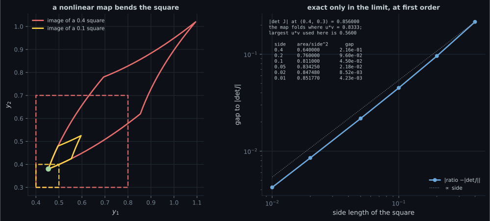
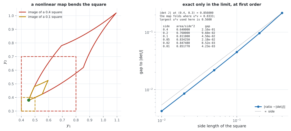
That word “approximates” carries the whole caveat, and the second figure below measures exactly how much of one.

From the book

Section 5.3. Definition 5.6 (Equation 5.58) gives the Jacobian as an $m\times n$ matrix of all first-order partials, with a margin note that the gradient of $f:\mathbb{R}^n\to\mathbb{R}^m$ is a matrix of size $m\times n$; a following remark notes that $f:\mathbb{R}^n\to\mathbb{R}^1$ is the special case of Equation 5.40. A Remark states that the book uses the numerator layout, whose transpose is the denominator layout. Equations 5.60 and 5.61 compute the areas of the unit square and of the parallelogram spanned by $[-2,1]$ and $[1,1]$; Equation 5.62 gives the transformation matrix, Equations 5.63 to 5.66 recover it as a Jacobian from the coordinate form, and Figure 5.5 draws it — with the note that $\lvert\det\mathbf{J}\rvert = 3$ is the area magnifier and that the Jacobian determinant reappears in §6.7’s change of variables. Example 5.9 (Equations 5.67 to 5.68) shows $\mathrm{d}(\mathbf{A}\mathbf{x})/\mathrm{d}\mathbf{x} = \mathbf{A}$. Example 5.10 (Equations 5.69 to 5.74) applies the chain rule to $h = f\circ g$ with $f(\mathbf{x}) = \exp(x_1x_2^2)$ and $g(t) = (t\cos t, t\sin t)$, first noting the shapes $1\times2$ and $2\times1$ at Equation 5.73. Example 5.11 (Equations 5.75 to 5.84) derives the least-squares gradient $\partial L/\partial\boldsymbol{\theta} = -2\mathbf{e}^\top\boldsymbol{\Phi} \in\mathbb{R}^{1\times D}$, with a Remark that the same result follows without the chain rule for simple functions but that this becomes impractical for deep compositions.

Worked example by hand

Example 5.9 — the identity every linear layer uses

$f(\mathbf{x}) = \mathbf{A}\mathbf{x}$ with $f(\mathbf{x})\in\mathbb{R}^M$, $\mathbf{A}\in\mathbb{R}^{M\times N}$, $\mathbf{x}\in\mathbb{R}^N$.

Step 1 — the shape, before any calculus. Since $f:\mathbb{R}^N\to\mathbb{R}^M$, it follows that $\mathrm{d}f/\mathrm{d}\mathbf{x}\in\mathbb{R}^{M\times N}$. Doing this first catches most errors before they happen.

Step 2 — the entries.

$$f_i(\mathbf{x}) = \sum_{j=1}^{N}A_{ij}x_j \implies \frac{\partial f_i}{\partial x_j} = A_{ij} \tag{5.67}$$

because every term in that sum except the $j$-th is constant with respect to $x_j$.

Step 3 — collect.

$$\frac{\mathrm{d}f}{\mathrm{d}\mathbf{x}} = \begin{bmatrix}A_{11}&\cdots&A_{1N}\\ \vdots&&\vdots\\ A_{M1}&\cdots&A_{MN}\end{bmatrix} = \mathbf{A} \in \mathbb{R}^{M\times N} \tag{5.68}$$

The Jacobian of a linear map is the matrix itself. Verified numerically for shapes $4\times3$, $2\times5$, $3\times3$ and $5\times1$, each agreeing with $\mathbf{A}$ to about $10^{-10}$.

This is the single most-used derivative in machine learning. Every dense layer’s backward pass is this identity plus the chain rule.

Example 5.10 — the chain rule, with the shapes checked first

$h:\mathbb{R}\to\mathbb{R}$, $h(t) = (f\circ g)(t)$, with

$$f(\mathbf{x}) = \exp(x_1x_2^2),\qquad \mathbf{x} = \begin{bmatrix}x_1\\x_2\end{bmatrix} = g(t) = \begin{bmatrix}t\cos t\\ t\sin t\end{bmatrix} \tag{5.71-5.72}$$

The book notes the shapes before computing anything:

$$\frac{\partial f}{\partial\mathbf{x}} \in \mathbb{R}^{1\times2},\qquad \frac{\partial g}{\partial t}\in\mathbb{R}^{2\times1} \tag{5.73}$$

so their product is $1\times1$ — a scalar, as it must be for $h:\mathbb{R}\to\mathbb{R}$.

$$\frac{\mathrm{d}h}{\mathrm{d}t} = \frac{\partial f}{\partial\mathbf{x}}\frac{\partial\mathbf{x}}{\partial t} = \begin{bmatrix}\dfrac{\partial f}{\partial x_1} & \dfrac{\partial f}{\partial x_2}\end{bmatrix} \begin{bmatrix}\dfrac{\partial x_1}{\partial t}\\[6pt] \dfrac{\partial x_2}{\partial t}\end{bmatrix} \tag{5.74a}$$

Filling in the pieces:

$$= \begin{bmatrix}\exp(x_1x_2^2)\,x_2^2 & 2\exp(x_1x_2^2)\,x_1x_2\end{bmatrix} \begin{bmatrix}\cos t - t\sin t\\ \sin t + t\cos t\end{bmatrix}$$ $$= \exp(x_1x_2^2)\Bigl[x_2^2(\cos t - t\sin t) + 2x_1x_2(\sin t + t\cos t)\Bigr]$$

Checked against a central difference in $t$ at six values, agreeing to between $9\times10^{-12}$ and $9\times10^{-10}$ relative:

$t$	chain rule	central difference
$0.30$	$0.036476225$	$0.036476224$
$0.70$	$0.706288861$	$0.706288861$
$1.00$	$1.529376673$	$1.529376673$
$1.50$	$-3.602659477$	$-3.602659476$
$2.00$	$-0.486106309$	$-0.486106309$
$2.50$	$0.036977693$	$0.036977693$

Example 5.11 — the least-squares gradient

This is the one that Chapter 9 runs on. Given the linear model

$$\mathbf{y} = \boldsymbol{\Phi}\boldsymbol{\theta} \tag{5.75}$$

with $\boldsymbol{\theta}\in\mathbb{R}^D$ a parameter vector, $\boldsymbol{\Phi}\in\mathbb{R}^{N\times D}$ the input features and $\mathbf{y}\in\mathbb{R}^N$ the observations, define

$$L(\mathbf{e}) := \lVert\mathbf{e}\rVert^2,\qquad \mathbf{e}(\boldsymbol{\theta}) := \mathbf{y} - \boldsymbol{\Phi}\boldsymbol{\theta} \tag{5.76-5.77}$$

Shape first: $\partial L/\partial\boldsymbol{\theta}\in\mathbb{R}^{1\times D}$ (Equation 5.78). Then the chain rule:

$$\frac{\partial L}{\partial\boldsymbol{\theta}} = \frac{\partial L}{\partial\mathbf{e}}\frac{\partial\mathbf{e}}{\partial\boldsymbol{\theta}} \tag{5.79}$$

Using $\lVert\mathbf{e}\rVert^2 = \mathbf{e}^\top\mathbf{e}$ from §3.2,

$$\frac{\partial L}{\partial\mathbf{e}} = 2\mathbf{e}^\top \in \mathbb{R}^{1\times N}, \qquad \frac{\partial\mathbf{e}}{\partial\boldsymbol{\theta}} = -\boldsymbol{\Phi} \in \mathbb{R}^{N\times D} \tag{5.81-5.82}$$

so

$$\boxed{\;\frac{\partial L}{\partial\boldsymbol{\theta}} = -2\mathbf{e}^\top\boldsymbol{\Phi} = -2\underbrace{(\mathbf{y}^\top - \boldsymbol{\theta}^\top\boldsymbol{\Phi}^\top)}_{1\times N}\underbrace{\boldsymbol{\Phi}}_{N\times D} \in \mathbb{R}^{1\times D}\;} \tag{5.83}$$

Note how the shapes carry the derivation: $(1\times N)(N\times D) = 1\times D$, which is what Equation 5.78 predicted before any differentiating happened.

Verified for $N = 30$, $D = 4$: the analytic gradient $[-86.449975,\ 161.597514,\ 43.111249,\ 73.585580]$ agrees with a central-difference Jacobian to $9.3\times10^{-10}$ relative, the two forms of Equation 5.83 agree exactly (0.0e+00), and at the least-squares solution the gradient is $2.5\times10^{-14}$ — zero, as an optimum requires.

The book’s Remark — why bother with the chain rule

The same result follows without the chain rule by expanding $L_2(\boldsymbol{\theta}) := \lVert\mathbf{y}-\boldsymbol{\Phi}\boldsymbol{\theta}\rVert^2 = (\mathbf{y}-\boldsymbol{\Phi}\boldsymbol{\theta})^\top(\mathbf{y}-\boldsymbol{\Phi}\boldsymbol{\theta})$. This approach is still practical for simple functions like $L_2$ but becomes impractical for deep function compositions. That sentence is the entire justification for §5.6.

See it move

sketch The Jacobian as a local linear map p5.js Pause Restart

A grid in the domain, pushed through a map you can switch between linear and nonlinear. The amber parallelogram is what the Jacobian at the marked point predicts; the blue patch is where the map actually sends that square. Shrink the square and the two converge — that is the whole content of 'the Jacobian approximates the map locally'.

sketch One row per output p5.js Pause Restart

Pick the number of outputs and inputs and watch the Jacobian's shape follow. Each row is highlighted as you scrub through the outputs, and the readout names what that row means. The point is that the shape rule never changes: rows are outputs, columns are inputs.

From scratch

jacobian_from_scratch.py

import numpy as np
 
def numeric_jac(f, x, h=1e-6):
    """Definition 5.6: one column per input, one row per output."""
    x = np.asarray(x, dtype=float).ravel()
    f0 = np.asarray(f(x)).ravel()
    J = np.zeros((f0.size, x.size))              # (outputs, inputs) -- numerator layout
    for j in range(x.size):
        e = np.zeros_like(x)
        e[j] = h
        J[:, j] = (np.asarray(f(x + e)).ravel() - np.asarray(f(x - e)).ravel()) / (2 * h)
    return J
 
rng = np.random.default_rng(3)
 
print("Example 5.9: d(Ax)/dx = A")
for (M, N) in [(4, 3), (2, 5), (3, 3), (5, 1)]:
    A = rng.normal(size=(M, N))
    x = rng.normal(size=N)
    J = numeric_jac(lambda v: A @ v, x)
    print(f"  A is {M}x{N}  ->  df/dx is {J.shape}  and equals A to {np.abs(J - A).max():.1e}")
 
print()
print("Example 5.10: h(t) = exp(x1 x2^2) with x = (t cos t, t sin t)")
h_of_t = lambda t: np.exp((t * np.cos(t)) * (t * np.sin(t)) ** 2)
 
def dh_chain(t):
    x1, x2 = t * np.cos(t), t * np.sin(t)
    e = np.exp(x1 * x2 ** 2)
    df_dx = np.array([[e * x2 ** 2, e * 2 * x1 * x2]])              # 1 x 2, Eq 5.73
    dx_dt = np.array([[np.cos(t) - t * np.sin(t)],
                      [np.sin(t) + t * np.cos(t)]])                 # 2 x 1, Eq 5.73
    return float((df_dx @ dx_dt).item())                            # (1x2)(2x1) -> (1,1)
 
print(f"{'t':>6}  {'chain rule':>18}  {'central difference':>20}  {'rel gap':>10}")
for t in (0.3, 0.7, 1.0, 1.5, 2.0, 2.5):
    ch = dh_chain(t)
    hh = 1e-6
    nu = (h_of_t(t + hh) - h_of_t(t - hh)) / (2 * hh)
    print(f"{t:>6.2f}  {ch:>18.9f}  {nu:>20.9f}  {abs(ch-nu)/max(abs(ch),1e-12):>10.1e}")
 
print()
print("Example 5.11: the least-squares gradient")
rng = np.random.default_rng(11)
N, D = 30, 4
Phi = rng.normal(size=(N, D))
theta_true = rng.normal(size=D)
y = Phi @ theta_true + 0.3 * rng.normal(size=N)
theta = rng.normal(size=D)
 
L = lambda th: (y - Phi @ th) @ (y - Phi @ th)
e0 = y - Phi @ theta
ana = (-2 * e0 @ Phi).reshape(1, -1)                                # Eq 5.83
num = numeric_jac(lambda v: np.array([L(v)]), theta)
ana2 = (-2 * (y.T - theta.T @ Phi.T) @ Phi).reshape(1, -1)          # Eq 5.83, expanded
 
print(f"  shape {ana.shape}  -- Eq 5.78 predicted 1 x D with D = {D}")
print(f"  analytic {np.round(ana[0], 6)}")
print(f"  numeric  {np.round(num[0], 6)}")
print(f"  relative error {np.abs(ana - num).max() / np.abs(ana).max():.1e}")
print(f"  the two forms of Eq 5.83 agree to {np.abs(ana2 - ana).max():.1e}")
th_star = np.linalg.lstsq(Phi, y, rcond=None)[0]
print(f"  at the least-squares optimum the gradient is "
      f"{np.abs(-2 * (y - Phi @ th_star) @ Phi).max():.1e}")

output

Example 5.9: d(Ax)/dx = A
  A is 4x3  ->  df/dx is (4, 3)  and equals A to 9.2e-11
  A is 2x5  ->  df/dx is (2, 5)  and equals A to 1.9e-10
  A is 3x3  ->  df/dx is (3, 3)  and equals A to 2.9e-10
  A is 5x1  ->  df/dx is (5, 1)  and equals A to 4.7e-11
 
Example 5.10: h(t) = exp(x1 x2^2) with x = (t cos t, t sin t)
     t          chain rule    central difference     rel gap
  0.30         0.036476225           0.036476224     8.8e-10
  0.70         0.706288861           0.706288861     9.3e-12
  1.00         1.529376673           1.529376673     1.6e-11
  1.50        -3.602659477          -3.602659476     1.2e-10
  2.00        -0.486106309          -0.486106309     4.4e-11
  2.50         0.036977693           0.036977693     3.5e-10
 
Example 5.11: the least-squares gradient
  shape (1, 4)  -- Eq 5.78 predicted 1 x D with D = 4
  analytic [-86.449975 161.597514  43.111249  73.58558 ]
  numeric  [-86.449975 161.597514  43.111249  73.58558 ]
  relative error 9.3e-10
  the two forms of Eq 5.83 agree to 0.0e+00
  at the least-squares optimum the gradient is 2.5e-14

Three things.

The shape line for Example 5.11 is the point of doing Equation 5.78 first: the gradient came out $(1, 4)$ exactly as predicted, and if it had come out $(4, 1)$ you would know immediately that a transpose went the wrong way — before looking at a single number.

The two forms of Equation 5.83 agree to 0.0e+00, exactly. That is not luck: $-2\mathbf{e}^\top\boldsymbol{\Phi}$ and $-2(\mathbf{y}^\top - \boldsymbol{\theta}^\top\boldsymbol{\Phi}^\top)\boldsymbol{\Phi}$ are the same floating-point operations in the same order once $\mathbf{e} = \mathbf{y}-\boldsymbol{\Phi}\boldsymbol{\theta}$ is substituted.

And at the least-squares solution the gradient is $2.5\times10^{-14}$ — which is the condition Chapter 9 solves for. Setting Equation 5.83 to zero gives $\boldsymbol{\Phi}^\top\boldsymbol{\Phi}\boldsymbol{\theta} = \boldsymbol{\Phi}^\top\mathbf{y}$, the normal equations.

On real data

figure The book's Figure 5.5, with the area counted matplotlib

The unit square maps to the parallelogram spanned by c1 = [-2,1] and c2 = [1,1]. det J = -3.0000, so |det J| = 3. A Monte-Carlo estimate over 400000 samples gives 3.0049 from 200329 hits, a gap of 0.0049 — the determinant claim verified by counting rather than by quoting §4.1. Note the sign: det is negative, so orientation flips.

figure 'Approximates locally', measured matplotlib

At (0.4, 0.3) the Jacobian determinant is 0.856000. The measured area ratio converges to it as the square shrinks: 0.640 at side 0.4, 0.811 at 0.1, 0.852 at 0.01 — with the gap falling in exact proportion to the side length, so the approximation is first order.

figure Definition 5.6's one rule, and every special case of it matplotlib

Rows indexed by the output, columns by the input — the numerator layout. Everything the chapter differentiates is this one rule: m = 1 gives §5.2's row, n = 1 gives a column, f(x) = Ax gives A itself, and a matrix argument gives a fourth-order tensor.

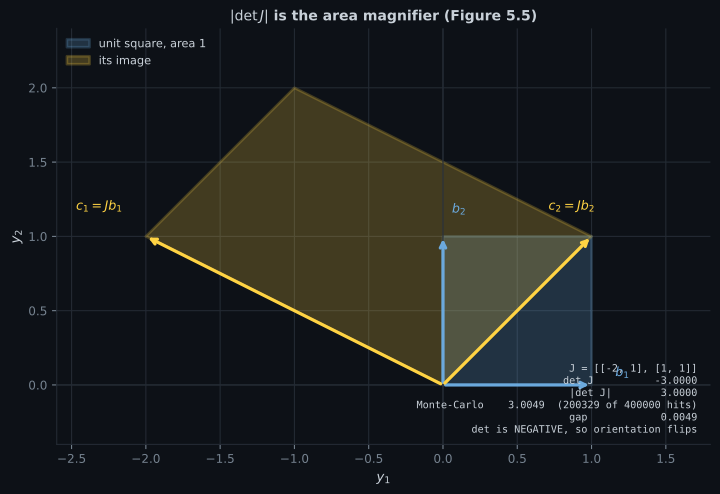
Reading the plot

From the area figure. The determinant is $-3$ and the area ratio is $3$, and both facts matter. The magnitude is the magnifier; the sign says the map reverses orientation, which the picture shows by $\mathbf{c}_1$ and $\mathbf{c}_2$ being swapped in handedness relative to $\mathbf{b}_1$ and $\mathbf{b}_2$.

The Monte-Carlo estimate is $3.0049$ against an exact $3$, from $200\,329$ hits out of $400\,000$. The gap of $0.0049$ is sampling noise — $\sigma \approx \text{box area}\sqrt{p(1-p)/n} \approx 0.005$ — so this is a check that passes, not a discrepancy. It matters because the estimate never touches the determinant: it counts points inside the image using coordinates in the $(\mathbf{b}_1,\mathbf{b}_2)$ frame, so agreement is independent evidence rather than a restatement.

From the local figure. This is the figure that puts a number on the word “approximates”. The gap between the measured area ratio and $\lvert\det\mathbf{J}\rvert$:

side	area / side²	gap
$0.4$	$0.640000$	$2.16\times10^{-1}$
$0.2$	$0.760000$	$9.60\times10^{-2}$
$0.1$	$0.811000$	$4.50\times10^{-2}$
$0.05$	$0.834250$	$2.18\times10^{-2}$
$0.02$	$0.847480$	$8.52\times10^{-3}$
$0.01$	$0.851770$	$4.23\times10^{-3}$

Every halving of the side halves the gap. First order — which is exactly what you should expect, because the Jacobian is the best linear approximation and the error is dominated by the first neglected term.

Note the base point: $(0.4, 0.3)$, not somewhere arbitrary. This map’s determinant is $1 - 1.2uv$, which vanishes on the hyperbola $uv = 0.8333$. Base the squares at $(0.8, 0.6)$ instead and the largest one reaches $uv = 1.2$, past the fold — and then the shoelace formula returns the difference of two oppositely-oriented areas rather than the area, giving a measured ratio of $0.04$ against a determinant of $0.424$. That is not a convergence failure; it is a folded polygon, and the figure avoids it deliberately.

From the shapes figure. The row worth pausing on is the last: a matrix argument gives a fourth-order tensor. §5.4 is about making that computable, and the figure previews the two ways — flatten, or partition into blocks.

Pitfalls

Check the layout convention before transposing anything

Numerator layout gives $m\times n$; denominator layout gives $n\times m$. They are transposes, and for a square Jacobian the shape cannot tell them apart. The book uses numerator layout; PyTorch’s autograd effectively produces gradients shaped like the parameter, which is the denominator convention for a scalar loss. Both produce code that runs. Read a non-square example before assuming.

A vanishing Jacobian determinant is not a small number, it is a different regime

Where $\det\mathbf{J} = 0$ the map is locally non-invertible: it collapses a direction. Past that surface it may fold, mapping two regions onto the same place — and then any area computed by a signed formula counts them with opposite signs. Measured above: a ratio of $0.04$ against a determinant of $0.424$, which looks like a broken convergence and is actually a broken assumption. Chapter 6’s change-of-variables formula requires an invertible transformation for exactly this reason.

The Jacobian of a linear map is constant; of a nonlinear map it is not

For $f(\mathbf{x}) = \mathbf{A}\mathbf{x}$ the Jacobian is $\mathbf{A}$ everywhere, so the linear preset in the first sketch has zero gap at every side length. For anything nonlinear the Jacobian is a function of position, and quoting “the Jacobian” without a point is meaningless.

Do the shape arithmetic before the calculus

Both Example 5.10 and Example 5.11 state the shapes first — Equations 5.73 and 5.78 — and then compute. That ordering catches nearly every error a chain rule can make, because a wrong transpose usually produces a shape that does not compose at all. When it does compose, as with a square Jacobian, you have lost your cheapest check.

A (1,1) NumPy array is not a Python float

(1×2) @ (2×1) gives shape (1,1), and float() of it raises TypeError on current NumPy. That is the shapes composing correctly. Use .item(), or index it. The temptation is to flatten the operands to 1-D to avoid the issue, which throws away the shape checking that made Equation 5.73 worth stating.

Compare

function	Jacobian	shape	note
$f:\mathbb{R}^n\to\mathbb{R}^m$	$\partial f_i/\partial x_j$	$m\times n$	Definition 5.6, the general rule
$f:\mathbb{R}^n\to\mathbb{R}$	the gradient	$1\times n$	§5.2’s Equation 5.40
$f:\mathbb{R}\to\mathbb{R}^m$	a column	$m\times1$	a curve’s velocity
$f(\mathbf{x}) = \mathbf{A}\mathbf{x}$	$\mathbf{A}$	$M\times N$	Example 5.9, constant everywhere
$f(\mathbf{x}) = \mathbf{x}$	$\mathbf{I}$	$n\times n$	$\det = 1$: no stretching
a rotation	the rotation matrix	$n\times n$	$\det = +1$: no stretching, no flip
$L(\boldsymbol{\theta}) = \lVert\mathbf{y}-\boldsymbol{\Phi}\boldsymbol{\theta}\rVert^2$	$-2\mathbf{e}^\top\boldsymbol{\Phi}$	$1\times D$	Example 5.11, Chapter 9’s gradient

pch.quizTag Check your understanding

1. Why does §5.3 add so little to §5.2?

   A Because vector-valued functions are rare B Because §5.2 already chose the row convention, so a function with m outputs is just m of those rows stacked — the shape rule 'rows are outputs, columns are inputs' extends with nothing to transpose C Because the Jacobian is the same as the gradient D Because it only covers linear functions
   pch.quizShowAnswer

   B — Because §5.2 already chose the row convention, so a function with m outputs is just m of those rows stacked — the shape rule 'rows are outputs, columns are inputs' extends with nothing to transpose — Definition 5.6 with m = 1 IS Equation 5.40. The book says so in a remark right after the definition. That is the payoff the row convention was chosen for.

2. The Monte-Carlo area estimate in the first figure came out as 3.0049 against an exact 3. Why is that worth showing rather than just quoting det J = -3?

   A It is not worth showing B Because the estimate never touches the determinant — it counts sampled points inside the image using coordinates in the original basis, so agreement is independent evidence rather than a restatement of §4.1 C Because the determinant is only approximate D Because Monte-Carlo is more accurate
   pch.quizShowAnswer

   B — Because the estimate never touches the determinant — it counts sampled points inside the image using coordinates in the original basis, so agreement is independent evidence rather than a restatement of §4.1 — The 0.0049 gap is sampling noise of the expected size for 400000 samples. A check that shares no code with the thing being checked is worth more than a tighter one that does.

3. For a nonlinear map, the measured area ratio approached |det J| with the gap halving each time the side halved. What does that exponent tell you?

   A That the measurement is imprecise B That the approximation is first order, which is what a LINEAR approximation must be — the error is dominated by the first neglected term, the quadratic one C That the Jacobian is wrong away from the point D That the map is not differentiable
   pch.quizShowAnswer

   B — That the approximation is first order, which is what a LINEAR approximation must be — the error is dominated by the first neglected term, the quadratic one — 0.216, 0.096, 0.045, 0.0218, 0.00852, 0.00423 as the side goes 0.4 down to 0.01 — proportional to the side throughout. 'The Jacobian approximates the map locally' has a rate, and this is it.

4. In the same figure, basing the squares at (0.8, 0.6) gave a measured ratio of 0.04 against a determinant of 0.424. What went wrong?

   A The convergence failed B Nothing about the calculus. det J = 1 - 1.2uv vanishes at uv = 0.8333 and that square reaches uv = 1.2, so the map FOLDS — and a signed area formula counts the two folded halves with opposite signs. The assumption broke, not the derivative C The determinant was computed at the wrong point D The square was too large for any Jacobian to help
   pch.quizShowAnswer

   B — Nothing about the calculus. det J = 1 - 1.2uv vanishes at uv = 0.8333 and that square reaches uv = 1.2, so the map FOLDS — and a signed area formula counts the two folded halves with opposite signs. The assumption broke, not the derivative — This is why Chapter 6's change-of-variables formula requires an invertible transformation. Where the Jacobian determinant vanishes you are not in a regime where 'volume magnifier' means anything.

5. Example 5.11 states the shape 1 x D before doing any calculus. What does that buy?

   A Nothing; it is a formality B The cheapest possible error check: a wrong transpose usually produces shapes that do not compose at all, so the mistake surfaces before any arithmetic. The derivation then just fills in a (1 x N)(N x D) product C It determines the numerical accuracy D It proves the gradient exists
   pch.quizShowAnswer

   B — The cheapest possible error check: a wrong transpose usually produces shapes that do not compose at all, so the mistake surfaces before any arithmetic. The derivation then just fills in a (1 x N)(N x D) product — And note where the check stops working: for a square Jacobian the shape composes either way, so you lose it. That is also when the numerator and denominator layouts become indistinguishable by shape.

🧪 Try It Yourself

Exercise 1 – Example 5.9, at four shapes

pch.exerciseTag pch.exerciseTitle

Exercise 2 – Example 5.10, shapes first

pch.exerciseTag pch.exerciseTitle

Exercise 3 – Example 5.11, and the normal equations

pch.exerciseTag pch.exerciseTitle

Exercise 4 – The determinant as an area magnifier

pch.exerciseTag pch.exerciseTitle

Exercise 5 – ‘Locally’ has a rate, and a boundary

pch.exerciseTag pch.exerciseTitle

Recall card

• The Jacobian is m gradient rows stacked: an m by n matrix with J(i,j) = the partial of output i with respect to input j — Definition 5.6, Equation 5.58.
• §5.2 was this with m = 1. Equation 5.40’s row vector is Definition 5.6’s special case, which is the payoff for choosing rows.
• Numerator layout means rows are outputs; the denominator layout is its transpose. They differ unless the Jacobian is square — and when it is square, the shape cannot tell them apart.
• The Jacobian of a linear map is the matrix itself, everywhere. Verified at four shapes, agreeing to about 1e-10.
• |det J| is the volume magnifier. For the book’s Figure 5.5, det J = −3 so areas triple and orientation flips; a Monte-Carlo count over 400000 samples gives 3.0049.
• For a nonlinear map that is only local, and the rate is first order. Measured: the gap between the area ratio and |det J| halves each time the side halves — 0.216 at side 0.4 down to 0.0042 at 0.01.
• Where det J = 0 the map folds, and a signed area formula then counts two halves against each other. That is why Chapter 6’s change of variables requires invertibility.
• The chain rule is a matrix product whose shapes are stated first. Equation 5.73 gives (1×2)(2×1); Equation 5.78 gives 1×D before any calculus happens.
• The least-squares gradient is −2 e-transpose Phi, shape 1 by D — Example 5.11, and Chapter 9’s whole starting point. Setting it to zero gives the normal equations.
• A (1,1) NumPy array is not a float. float() on it raises, and that is the shapes composing correctly. Use .item().

Next: Gradients of Matrices — where the derivative becomes a fourth-order tensor, and the two ways to make that computable.