Probabilistic Modeling and Inference

Page 805 ended on the book’s own limit: MAP “still only produces a point estimate of the parameters.” You write down an entire posterior distribution and then keep the location of its peak.

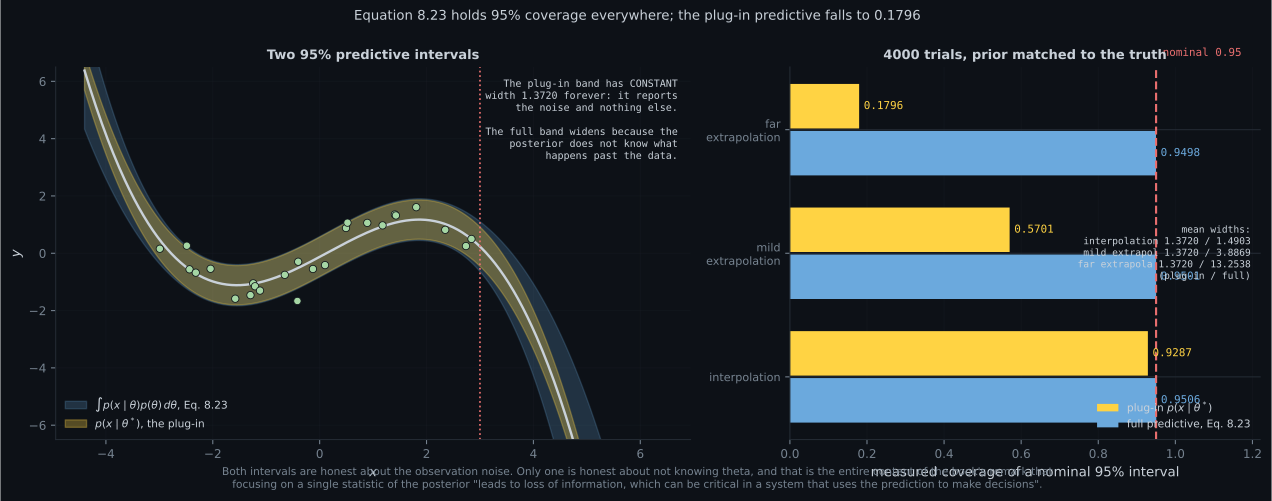
This page keeps the rest. And it measures what that buys, because the difference is not philosophical: a nominal 95% interval built from the full posterior achieves 0.9506, 0.9501 and 0.9498 coverage across three regions, while the plug-in interval built from the point estimate achieves 0.9287, 0.5701 and 0.1796.

What you’ll learn

• Why §8.4.1 says a probabilistic model is specified by the joint distribution — and what “only the joint distribution has this property” means.
• Equation 8.22, and the integral in its denominator that MAP was allowed to skip.
• Equation 8.23: predictions become an average over all plausible parameters, measured to hold 95% coverage where the plug-in falls to 0.1796.
• The book’s own comparison: estimation is an optimization problem, inference is an integration problem — and when the difference stops mattering (measured: at $N = 10000$ the two intervals differ by a factor of $1.000113$).
• §8.4.3 latent variables, and Equation 8.25’s insistence that the likelihood “must not depend on” $\mathbf{z}$.
• The honest limit, measured: on the chapter’s misspecified sine data, the full predictive reaches only $0.8908$. Bayesian inference quantifies doubt about $\boldsymbol\theta$, not doubt about the model class.

Intuition: the difference between a guess and a guess with a margin

You fit a model and it predicts $137.46$. Two follow-up questions:

1. Would you bet on it?
2. Would you bet on it for an input nothing like the training data?

A point estimate cannot answer either. It hands back one number, and any interval you attach comes from the noise term $\sigma^2$ alone — a constant, the same width at the centre of the data and a hundred units outside it. That is the plug-in predictive $p(x \mid \boldsymbol\theta^*)$, and it is structurally incapable of saying “I don’t know”.

The posterior can. It holds many parameter vectors, all consistent with the data. Where the data pins them down, they agree and the prediction is tight. Where the data says nothing, they disagree wildly and the prediction is wide. That disagreement is the uncertainty, and Equation 8.23 is the instruction to report it.

The price is an integral. Optimization finds a peak; integration sums over everything. That is the book’s whole comparison in one line.

diagram Two problems, two costs mermaid

  flowchart TD
  J["the JOINT p(x, theta)
Section 8.4.1: this IS the model"]
  J -->|"product rule"| PL["prior x likelihood"]
  J -->|"sum rule, integrate out theta"| ML["marginal likelihood p(x)
Section 8.6 needs this"]
  J -->|"divide by p(x)"| PO["posterior p(theta | x)"]
  PO --> EST["Section 8.3: keep the PEAK
problem = OPTIMIZATION
answer = a point"]
  PO --> INF["Section 8.4.2: keep it ALL
problem = INTEGRATION
answer = a distribution"]
  EST --> P1["p(x | theta*)
width 1.3720 forever
far-extrap coverage 0.1796"]
  INF --> P2["Eq 8.23: average over theta
width grows with doubt
far-extrap coverage 0.9498"]

§8.4.1 Probabilistic models

The book’s framing: probabilistic models “represent the uncertain aspects of an experiment as probability distributions”, and the benefit is “a unified and consistent set of tools from probability theory for modeling, inference, prediction, and model selection” — one toolkit for all four jobs.

The central object is the joint distribution $p(\mathbf{x}, \boldsymbol\theta)$ of the observed variables and the hidden parameters, because it “encapsulates information from the following”:

what you want	how the joint gives it	which rule (§6.3)
the prior and the likelihood	they are its factors	product rule
the marginal likelihood $p(\mathbf{x})$	integrate out $\boldsymbol\theta$	sum rule
the posterior	divide the joint by the marginal	—

And then the sentence that justifies the whole framing:

Only the joint distribution has this property. Therefore, a probabilistic model is specified by the joint distribution of all its random variables.

That is a definition, not a remark. A probabilistic model is a joint distribution. Everything else — prior, likelihood, posterior, evidence — is something you derive from it by applying a rule of probability. This is why §8.5’s graphical language is about the joint and nothing else.

§8.4.2 Bayesian inference

For a dataset $\mathcal{X}$, a parameter prior $p(\boldsymbol\theta)$, and a likelihood function, the posterior is

$$p(\boldsymbol\theta \mid \mathcal{X}) = \frac{p(\mathcal{X} \mid \boldsymbol\theta)\,p(\boldsymbol\theta)}{p(\mathcal{X})}, \qquad p(\mathcal{X}) = \int p(\mathcal{X} \mid \boldsymbol\theta)\,p(\boldsymbol\theta)\,d\boldsymbol\theta$$

The key idea, in the book’s words, is “to exploit Bayes’ theorem to invert the relationship between the parameters $\boldsymbol\theta$ and the data $\mathcal{X}$”. The likelihood runs parameters → data; the posterior runs data → parameters.

Note the denominator. Page 805’s MAP estimation could drop $p(\mathcal{X})$ because it is constant in $\boldsymbol\theta$. Bayesian inference cannot: it needs the posterior normalised, so it needs that integral. This one difference is the source of essentially every practical difficulty on this page.

Equation 8.23: predictions stop depending on the parameters

With a distribution on the parameters, the prediction becomes

$$p(\mathbf{x}) = \int p(\mathbf{x} \mid \boldsymbol\theta)\,p(\boldsymbol\theta)\,d\boldsymbol\theta = \mathbb{E}_{\boldsymbol\theta}\!\left[p(\mathbf{x} \mid \boldsymbol\theta)\right]$$

The parameters have been marginalised out. The book: “the prediction is an average over all plausible parameter values $\boldsymbol\theta$, where the plausibility is encapsulated by the parameter distribution.”

For a Gaussian model this has a closed form worth memorising. At an input $\boldsymbol\phi$:

$$\text{mean} = \boldsymbol\phi^\top\mathbf{m}_N, \qquad \text{variance} = \underbrace{\sigma^2}_{\text{noise}} + \underbrace{\boldsymbol\phi^\top\boldsymbol\Sigma_N\boldsymbol\phi}_{\text{not knowing }\boldsymbol\theta}$$

The mean is the same as the plug-in prediction. Only the variance differs — and only by that second term, which is exactly what the point estimate discarded.

The variance split, measured

$x$	noise	parameters	total	parameter share
$0.0$	$0.122500$	$0.009862$	$0.132362$	$7.5\%$
$2.0$	$0.122500$	$0.016043$	$0.138543$	$11.6\%$
$3.0$	$0.122500$	$0.073805$	$0.196305$	$37.6\%$
$4.0$	$0.122500$	$0.543523$	$0.666023$	$81.6\%$
$5.0$	$0.122500$	$2.464844$	$2.587344$	$95.3\%$

The training data spans $-3$ to $3$. Inside it the noise dominates and the two predictives barely differ. Two units outside it, $81.6\%$ of the uncertainty is not knowing $\boldsymbol\theta$ — which is precisely the part the plug-in predictive reports as zero.

Why it matters: the book’s argument, measured

The book’s case is about decisions:

Focusing solely on some statistic of the posterior distribution (such as the parameter $\boldsymbol\theta^*$ that maximizes the posterior) leads to loss of information, which can be critical in a system that uses the prediction $p(\mathbf{x} \mid \boldsymbol\theta^*)$ to make decisions.

To measure “critical”, I drew $\boldsymbol\theta$ from the prior, drew data from the model, and counted how often a nominal $95\%$ interval actually contained the held-out value — $4000$ trials, $160{,}000$ test points per region.

Coverage of a nominal 95% interval, 4000 trials

region	plug-in coverage	Eq. 8.23 coverage	plug-in width	full width
interpolation, $-3$ to $3$	$0.9287$	$\mathbf{0.9506}$	$1.3720$	$1.4903$
mild extrapolation, $3$ to $5$	$0.5701$	$\mathbf{0.9501}$	$1.3720$	$3.8869$
far extrapolation, $5$ to $7$	$\mathbf{0.1796}$	$\mathbf{0.9498}$	$1.3720$	$13.2538$

Equation 8.23 holds $0.95$ everywhere. The plug-in interval is a near miss inside the data and catastrophic outside it: in far extrapolation it covers the truth 18% of the time while claiming 95%.

Its width is $1.3720$ in all three rows, because $2 \times 1.96 \times \sigma$ does not depend on where you ask. That constant is the entire failure.

This is the setting where the Bayesian interval is guaranteed correct: the prior is the truth. That guarantee is what is being verified, and it holds to three decimal places.

Estimation against inference, as the book puts it

	parameter estimation (§8.3)	Bayesian inference (§8.4.2)
what you get	“a consistent point estimate” $\boldsymbol\theta^*$	“a (posterior) distribution”
computational problem	optimization	integration
making a prediction	“straightforward”	“require solving another integration problem”
prior knowledge	not easily incorporated	“a principled way”
structural/side information	hard	“not easily done” the other way
uncertainty propagation	none	valuable for “risk assessment and exploration”

The book cites the payoff in “data-efficient learning” (Deisenroth et al., 2015; Kamthe and Deisenroth, 2018) — knowing what you don’t know is what tells you where to look next.

When the gap closes

Measured on the chapter’s own data, with the posterior recomputed at each sample size:

$N$	largest posterior sd	full interval / plug-in width
$5$	$0.821958$	$1.248213$
$10$	$0.806301$	$1.116420$
$25$	$0.392692$	$1.039472$
$100$	$0.239610$	$1.011311$
$1000$	$0.074293$	$1.001109$
$10000$	$0.022878$	$\mathbf{1.000113}$

At $N = 10000$ the two intervals differ by one part in nine thousand. This is why maximum likelihood is defensible on large data and reckless on small data — and it is the same $1/\sqrt{N}$ collapse page 804 measured from the frequentist side.

The practical obstacle

The book is direct about the cost:

If we do not choose a conjugate prior on the parameters (§6.6.1), the integrals in (8.22) and (8.23) are not analytically tractable, and we cannot compute the posterior, the predictions, or the marginal likelihood in closed form.

Everything on this page is computed exactly because the prior is conjugate. Step outside that and you need approximations. The book’s list, grouped:

kind	methods
stochastic	Markov chain Monte Carlo (Gilks et al., 1996)
deterministic	the Laplace approximation; variational inference (Jordan et al., 1999; Blei et al., 2017); expectation propagation (Minka, 2001a)

And the applications where the cost was judged worth paying: “large-scale topic modeling, click-through-rate prediction, data-efficient reinforcement learning in control systems, online ranking systems, and large-scale recommender systems”, plus Bayesian optimization as a “generic tool” for “efficient search of meta parameters”.

The book’s remark on variables versus parameters

The book notes that the split between “(random) ‘variables’” and “parameters” is “somewhat arbitrary” — parameters get estimated, variables get marginalised out. But “in principle, we can place a prior on any parameter and integrate it out, which would then turn the parameter into a random variable”. The distinction describes what you chose to do, not what the object is.

§8.4.3 Latent-variable models

Latent variables $\mathbf{z}$ are “different from the model parameters $\boldsymbol\theta$ as they do not parametrize the model explicitly”. They exist because they “may describe the data-generating process, thereby contributing to the interpretability of the model” and because they “often simplify the structure of the model” — usually with fewer parameters, not more.

The generative direction is Equation 8.24:

$$p(\mathbf{x} \mid \boldsymbol\theta, \mathbf{z})$$

and since $\mathbf{z}$ is latent, it gets a prior $p(\mathbf{z})$.

Learning then proceeds in two steps. First compute a likelihood that does not mention $\mathbf{z}$; second, feed it to §8.3 or §8.4.2 unchanged. The first step is Equation 8.25:

$$p(\mathbf{x} \mid \boldsymbol\theta) = \int p(\mathbf{x} \mid \boldsymbol\theta, \mathbf{z})\,p(\mathbf{z})\,d\mathbf{z}$$

with the book’s insistence in the margin: “Note that the likelihood must not depend on the latent variables $\mathbf{z}$, but it is only a function of the data $\mathbf{x}$ and the model parameters $\boldsymbol\theta$.”

Equation 8.25 on a two-component mixture, measured

Latent $z \in \{0, 1\}$ with $p(z) = (0.3, 0.7)$, and $p(x \mid z)$ Gaussian at $-1.5$ and $2.0$:

$x$	$p(x \mid z{=}0)$	$p(x \mid z{=}1)$	$p(x)$, marginalised	$p(z{=}0 \mid x)$
$-2.0$	$0.410201$	$0.000000$	$0.123060$	$1.000000$
$0.0$	$0.085983$	$0.000268$	$0.025982$	$0.992789$
$1.9$	$0.000060$	$0.782085$	$0.547478$	$0.000033$
$3.0$	$0.000000$	$0.107982$	$0.075587$	$0.000000$

The marginal integrates to $1.00000000$ over $x$. It is a density in $x$ and does not mention $z$ at all — which is exactly the book’s note. The last column is Equation 8.28, the posterior on the latent given the data and the parameters.

The book lists where this pays: “principal component analysis for dimensionality reduction (Chapter 10), Gaussian mixture models for density estimation (Chapter 11), hidden Markov models or dynamical systems for time-series modeling, and meta learning and task generalization”. It also gives the warning up front: “learning in latent-variable models is generally hard, as we will see in Chapter 11”, with the EM algorithm (Dempster et al., 1977) as the principled route via maximum likelihood.

Three posteriors, in order of difficulty

what you want	equation	what it costs
$p(\boldsymbol\theta \mid \mathcal{X})$, parameters	8.26	needs Eq. 8.25’s integral over $\mathbf{z}$ first
$p(\mathbf{z} \mid \mathcal{X})$, latents	8.27	needs $p(\mathcal{X} \mid \mathbf{z}) = \int p(\mathcal{X} \mid \mathbf{z}, \boldsymbol\theta)p(\boldsymbol\theta)d\boldsymbol\theta$
both at once	—	“not possible in general”
$p(\mathbf{z} \mid \mathcal{X}, \boldsymbol\theta)$, latents given parameters	8.28	“a quantity that is easier to compute”

The last row is the practical compromise, and it is not an accident that Chapters 10 and 11 compute exactly Equation 8.28 for PCA and for Gaussian mixture models. When both integrals are intractable, you condition on one instead of integrating it.

§8.4.4 Further reading

Ghahramani (2015) gives “a short review of probabilistic models in machine learning”. Moustaki et al. (2015) and Paquet (2008) cover Bayesian inference in latent-variable models. And the book flags a field built around automating all of this:

Several programming languages have been proposed that aim to treat the variables defined in software as random variables corresponding to probability distributions. The objective is to be able to write complex functions of probability distributions, while under the hood the compiler automatically takes care of the rules of Bayesian inference. This rapidly changing field is called probabilistic programming.

Worked example by hand

The Gaussian mean again — the smallest case where you can watch a posterior appear.

Model: $y_n \sim \mathcal{N}(\theta, \sigma^2)$, $N$ observations, prior $\theta \sim \mathcal{N}(0, \tau^2)$.

Step 1: the posterior is Gaussian, so find its two numbers. Collect the $\theta$-dependent part of the negative log-posterior:

$$\frac{1}{2\sigma^2}\sum_n (y_n - \theta)^2 + \frac{\theta^2}{2\tau^2} = \frac{1}{2}\theta^2\left(\frac{N}{\sigma^2} + \frac{1}{\tau^2}\right) - \theta\,\frac{N\bar{y}}{\sigma^2} + \text{const}$$

A quadratic in $\theta$ is a Gaussian. Matching to $\frac{1}{2\sigma_N^2}(\theta - m_N)^2$:

$$\boxed{\ \frac{1}{\sigma_N^2} = \frac{N}{\sigma^2} + \frac{1}{\tau^2}, \qquad m_N = \sigma_N^2\,\frac{N\bar{y}}{\sigma^2}\ }$$

Step 2: read the precision. Precisions add: the data contributes $N/\sigma^2$ and the prior contributes $1/\tau^2$. Each observation adds exactly $1/\sigma^2$ of certainty, which is why the posterior sd falls like $1/\sqrt{N}$.

Step 3: check $m_N$ against page 805. Substituting $\sigma_N^2$:

$$m_N = \frac{N\bar{y}/\sigma^2}{N/\sigma^2 + 1/\tau^2} = \frac{N}{N + \sigma^2/\tau^2}\,\bar{y}$$

That is page 805’s MAP estimate exactly. For a Gaussian, the posterior mean and the MAP point coincide — so nothing about the location was lost. Everything lost was $\sigma_N^2$.

Step 4: build the predictive, Equation 8.23. A new observation is $y_{\text{new}} = \theta + \epsilon$ with $\theta \sim \mathcal{N}(m_N, \sigma_N^2)$ and $\epsilon \sim \mathcal{N}(0, \sigma^2)$ independent. A sum of independent Gaussians adds variances:

$$p(y_{\text{new}} \mid \mathcal{X}) = \mathcal{N}\!\left(m_N,\ \sigma^2 + \sigma_N^2\right)$$

Step 5: compare with the plug-in. The plug-in predictive is $\mathcal{N}(m_N, \sigma^2)$ — same centre, and missing $\sigma_N^2$ entirely. The ratio of interval widths is

$$\sqrt{1 + \frac{\sigma_N^2}{\sigma^2}} = \sqrt{1 + \frac{1}{N + \sigma^2/\tau^2}}$$

which tends to $1$ as $N$ grows and blows up as $N \to 0$. Optimization and integration agree in the limit of infinite data and disagree most exactly when you have least.

See it move

sketch One point, or the whole posterior p5.js Pause Restart

A Gaussian posterior over the mean of a small dataset. Drag the sample size and the prior width; watch the posterior narrow, the MAP point stay at its centre, and the gap between the plug-in predictive and the full predictive open and close.

From scratch

bayesian_inference.py

import numpy as np
 
SIGMA, TAU2, D = 0.35, 1.0, 4
Z = 1.959963984540054
 
def make(n, seed):
    rng = np.random.default_rng(seed)
    x = np.sort(rng.uniform(-3, 3, n))
    return x, np.sin(1.4 * x) + 0.3 * x + SIGMA * rng.standard_normal(n)
 
def design(x, deg=3):
    return np.vander(np.asarray(x, float) / 3.0, deg + 1, increasing=True)
 
x, y = make(25, seed=3)
Phi = design(x)
N = len(y)
 
# --- Equation 8.22: the exact posterior, by conjugacy (Section 6.6.1) ---
Sigma = np.linalg.inv(Phi.T @ Phi / SIGMA ** 2 + np.eye(D) / TAU2)
mean = Sigma @ Phi.T @ y / SIGMA ** 2
 
# the MAP estimate of Section 8.3.2, for comparison
mapest = np.linalg.solve(Phi.T @ Phi / SIGMA ** 2 + np.eye(D) / TAU2,
                         Phi.T @ y / SIGMA ** 2)
print("=== 1. the point estimate is the posterior MEAN ===")
print(f"posterior mean : {np.round(mean, 6).tolist()}")
print(f"MAP estimate   : {np.round(mapest, 6).tolist()}")
print(f"max difference : {np.abs(mean - mapest).max():.2e}")
print("MAP is not wrong -- it is incomplete. What it discarded:")
print(f"posterior sd   : {np.round(np.sqrt(np.diag(Sigma)), 6).tolist()}")
 
# --- Equation 8.23: the predictive averages over theta ------------------
print("\n=== 2. the variance of Equation 8.23 splits in two ===")
print(f"{'x':>6} {'noise':>10} {'parameters':>12} {'total':>10} {'share':>8}")
for xs in (0.0, 2.0, 3.0, 4.0, 5.0):
    q = design([xs])[0]
    pv = float(q @ Sigma @ q)
    print(f"{xs:>6.1f} {SIGMA**2:>10.6f} {pv:>12.6f} {SIGMA**2+pv:>10.6f} "
          f"{pv/(SIGMA**2+pv):>7.1%}")
print("inside the data the noise dominates; outside it the parameters do.")
 
# --- does it matter? calibration, with the prior matched to the truth ---
print("\n=== 3. coverage of a nominal 95% interval, 4000 trials ===")
rng = np.random.default_rng(11)
regions = (("interpolation", -3.0, 3.0), ("mild extrapolation", 3.0, 5.0),
           ("far extrapolation", 5.0, 7.0))
hp = {r[0]: 0 for r in regions}; hf = dict(hp); wf = {r[0]: 0.0 for r in regions}
tot = dict(hp)
for _ in range(4000):
    th = np.sqrt(TAU2) * rng.standard_normal(D)      # theta from the prior
    xtr = np.sort(rng.uniform(-3, 3, 25))
    P = design(xtr)
    ytr = P @ th + SIGMA * rng.standard_normal(25)   # data from the model
    C = np.linalg.inv(P.T @ P / SIGMA ** 2 + np.eye(D) / TAU2)
    m = C @ P.T @ ytr / SIGMA ** 2
    for name, lo, hi in regions:
        xt = rng.uniform(lo, hi, 40)
        Pt = design(xt)
        yt = Pt @ th + SIGMA * rng.standard_normal(len(xt))
        mu = Pt @ m
        sd = np.sqrt(SIGMA ** 2 + np.einsum("ij,jk,ik->i", Pt, C, Pt))
        hp[name] += int(np.sum(np.abs(yt - mu) <= Z * SIGMA))
        hf[name] += int(np.sum(np.abs(yt - mu) <= Z * sd))
        wf[name] += float(np.sum(2 * Z * sd))
        tot[name] += len(xt)
print(f"{'region':>20} {'plug-in':>9} {'Eq. 8.23':>9} {'plug width':>11} "
      f"{'full width':>11}")
for name, lo, hi in regions:
    n = tot[name]
    print(f"{name:>20} {hp[name]/n:>9.4f} {hf[name]/n:>9.4f} "
          f"{2*Z*SIGMA:>11.4f} {wf[name]/n:>11.4f}")
print("Equation 8.23 holds 0.95 everywhere. The plug-in interval reports")
print("only the noise, so it collapses the further it goes from the data.")
 
# --- as N grows, the two converge --------------------------------------
print("\n=== 4. optimization and integration converge as N grows ===")
q0 = design([0.0])[0]
print(f"{'N':>7} {'max post. sd':>14} {'width ratio full/plug':>23}")
for n in (5, 10, 25, 100, 1000, 10000):
    xn, yn = make(n, seed=3)
    Pn = design(xn)
    Cn = np.linalg.inv(Pn.T @ Pn / SIGMA ** 2 + np.eye(D) / TAU2)
    v = float(q0 @ Cn @ q0)
    print(f"{n:>7} {np.sqrt(np.diag(Cn)).max():>14.6f} "
          f"{np.sqrt((SIGMA**2+v)/SIGMA**2):>23.6f}")
print("the ratio tends to 1: with enough data a point estimate is fine.")
 
# --- p(X), the term MAP was allowed to drop ----------------------------
print("\n=== 5. the marginal likelihood p(X) ===")
def log_evidence(deg):
    P = design(x, deg)
    C = SIGMA ** 2 * np.eye(N) + TAU2 * (P @ P.T)
    _, ld = np.linalg.slogdet(C)
    return float(-0.5 * (y @ np.linalg.solve(C, y) + ld + N*np.log(2*np.pi)))
evs = [log_evidence(d) for d in range(12)]
kb = int(np.argmax(evs))
print(f"{'degree':>7} {'log p(X)':>11} {'Bayes factor vs best':>22}")
for d in range(12):
    print(f"{d:>7} {evs[d]:>11.4f} {np.exp(evs[d]-evs[kb]):>22.4f}")
print(f"peak at degree {kb}. Degree 11 is only "
      f"{evs[kb]-evs[11]:.4f} nats behind --")
print("the evidence penalises extra capacity but does not forbid it.")
 
# --- Equation 8.25: marginalising out a latent variable ----------------
print("\n=== 6. Equation 8.25: integrating out a latent variable ===")
pz = np.array([0.3, 0.7])
mus, sds = np.array([-1.5, 2.0]), np.array([0.8, 0.5])
def p_x_given_z(xs, k):
    return (np.exp(-0.5 * ((xs - mus[k]) / sds[k]) ** 2)
            / (sds[k] * np.sqrt(2 * np.pi)))
print(f"{'x':>6} {'p(x|z=0)':>11} {'p(x|z=1)':>11} {'p(x) marginal':>15} "
      f"{'p(z=0|x)':>10}")
for xs in (-2.0, 0.0, 1.9, 3.0):
    a, b = p_x_given_z(xs, 0), p_x_given_z(xs, 1)
    marg = pz[0] * a + pz[1] * b
    print(f"{xs:>6.1f} {a:>11.6f} {b:>11.6f} {marg:>15.6f} "
          f"{pz[0]*a/marg:>10.6f}")
grid = np.linspace(-12, 14, 2000001)
dens = pz[0] * p_x_given_z(grid, 0) + pz[1] * p_x_given_z(grid, 1)
print(f"area under the marginal: {np.trapezoid(dens, grid):.8f}")
print("the marginal is a density in x and does not mention z at all,")
print("which is the book's note beneath Equation 8.25.")

text

=== 1. the point estimate is the posterior MEAN ===
posterior mean : [-0.126578, 2.997457, 0.487525, -3.122058]
MAP estimate   : [-0.126578, 2.997457, 0.487525, -3.122058]
max difference : 8.88e-16
MAP is not wrong -- it is incomplete. What it discarded:
posterior sd   : [0.099305, 0.26664, 0.224268, 0.392692]
 
=== 2. the variance of Equation 8.23 splits in two ===
     x      noise   parameters      total    share
   0.0   0.122500     0.009862   0.132362    7.5%
   2.0   0.122500     0.016043   0.138543   11.6%
   3.0   0.122500     0.073805   0.196305   37.6%
   4.0   0.122500     0.543523   0.666023   81.6%
   5.0   0.122500     2.464844   2.587344   95.3%
inside the data the noise dominates; outside it the parameters do.
 
=== 3. coverage of a nominal 95% interval, 4000 trials ===
              region   plug-in  Eq. 8.23  plug width  full width
       interpolation    0.9287    0.9506      1.3720      1.4903
  mild extrapolation    0.5701    0.9501      1.3720      3.8869
   far extrapolation    0.1796    0.9498      1.3720     13.2538
Equation 8.23 holds 0.95 everywhere. The plug-in interval reports
only the noise, so it collapses the further it goes from the data.
 
=== 4. optimization and integration converge as N grows ===
      N   max post. sd   width ratio full/plug
      5       0.821958                1.248213
     10       0.806301                1.116420
     25       0.392692                1.039472
    100       0.239610                1.011311
   1000       0.074293                1.001109
  10000       0.022878                1.000113
the ratio tends to 1: with enough data a point estimate is fine.
 
=== 5. the marginal likelihood p(X) ===
 degree    log p(X)   Bayes factor vs best
      0   -100.7863                 0.0000
      1    -63.2439                 0.0000
      2    -61.4607                 0.0000
      3    -30.7910                 0.4362
      4    -31.0573                 0.3342
      5    -30.0952                 0.8746
      6    -29.9612                 1.0000
      7    -30.2679                 0.7359
      8    -30.1686                 0.8127
      9    -30.2674                 0.7363
     10    -30.2657                 0.7375
     11    -30.2178                 0.7737
peak at degree 6. Degree 11 is only 0.2566 nats behind --
the evidence penalises extra capacity but does not forbid it.
 
=== 6. Equation 8.25: integrating out a latent variable ===
     x    p(x|z=0)    p(x|z=1)   p(x) marginal   p(z=0|x)
  -2.0    0.410201    0.000000        0.123060   1.000000
   0.0    0.085983    0.000268        0.025982   0.992789
   1.9    0.000060    0.782085        0.547478   0.000033
   3.0    0.000000    0.107982        0.075587   0.000000
area under the marginal: 1.00000000
the marginal is a density in x and does not mention z at all,
which is the book's note beneath Equation 8.25.

On real data

figure Parameter estimation returns a point; Bayesian inference returns a distribution matplotlib

The posterior mean equals the MAP estimate to 8.88e-16, so the point estimate is not wrong — it is incomplete. Each of the forty curves explains the same twenty-five points. Their agreement inside the data and disagreement outside it is the uncertainty a point estimate cannot report.

figure Equation 8.23 holds 95 percent coverage everywhere; the plug-in predictive falls to 0.1796 matplotlib

Measured over 4000 trials with the prior matched to the truth. The plug-in band has width 1.3720 in every region because two times 1.96 times sigma does not depend on where you ask. In far extrapolation it covers the truth 18 percent of the time while claiming 95.

figure Estimation solves an optimization problem; inference solves an integration problem matplotlib

Only the parameter term vanishes with more data — the width ratio falls from 1.248213 at N equals 5 to 1.000113 at N equals 10000. The third panel is the marginal likelihood MAP was allowed to drop, and the quantity Section 8.6 needs in order to choose a model at all.

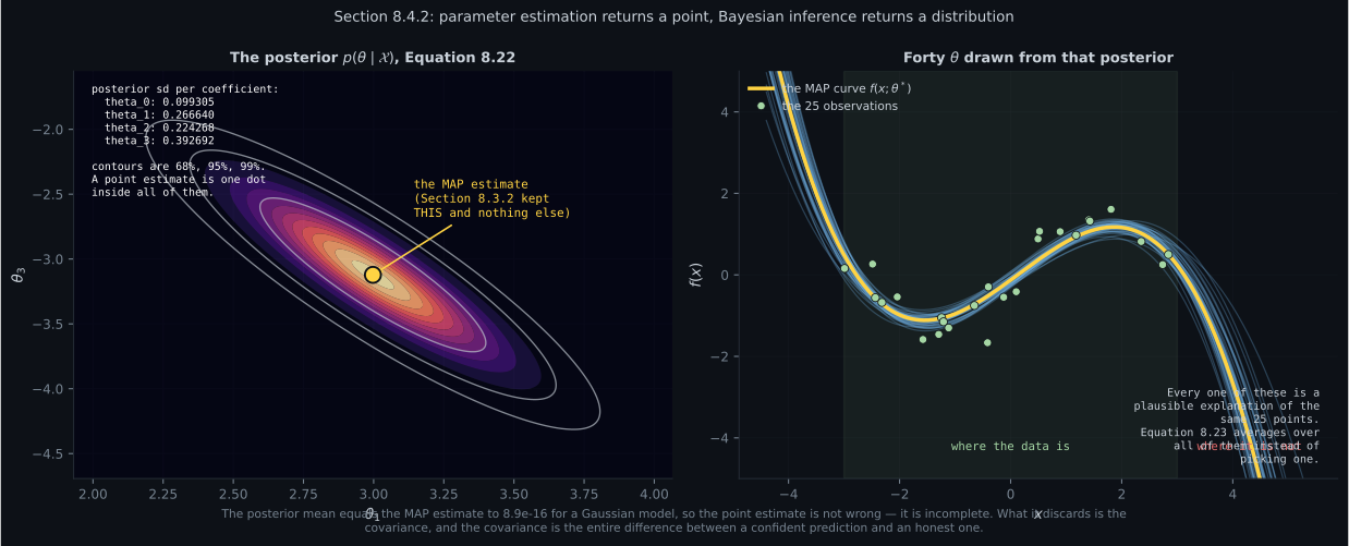
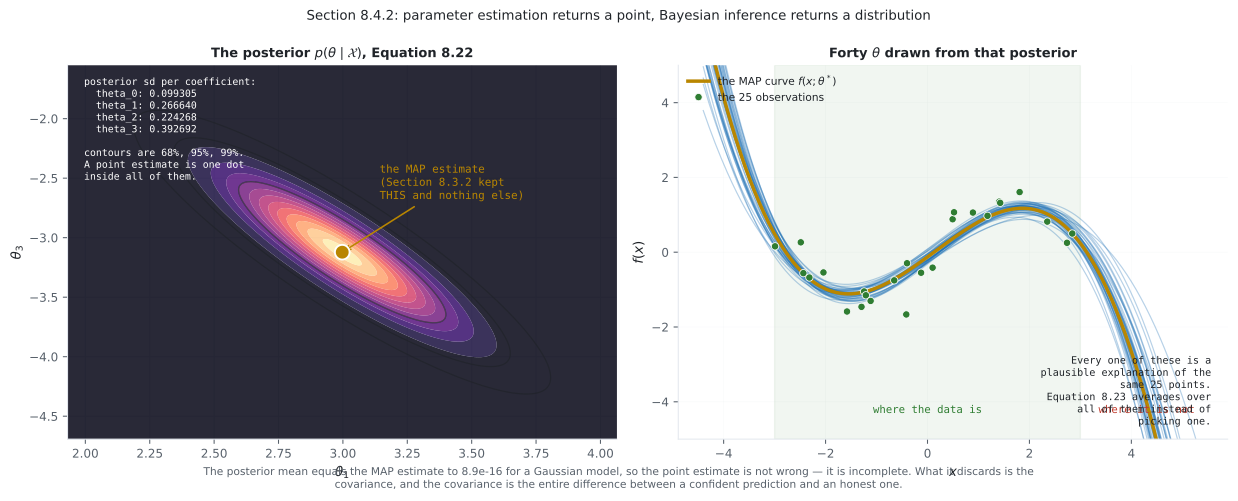
Reading the plot

The first figure is the whole of §8.4 in two panels. On the left, the posterior over two coefficients as a filled density with 68%, 95% and 99% contours, and the MAP estimate as a single dot. The dot sits at the distribution’s centre — measured, the posterior mean and the MAP estimate agree to $8.88\times10^{-16}$. The point estimate is not in the wrong place. It is simply one dot where there was a distribution.

The right panel shows what that costs. Forty parameter vectors drawn from the posterior, each plotted as a curve. Between $-3$ and $3$ they are indistinguishable — the data pins them down. Past $3$ they fan apart violently. Every one of those curves explains the same twenty-five observations equally well, and their disagreement is a measurement of ignorance, available for free once you have the covariance and unavailable forever once you have thrown it away.

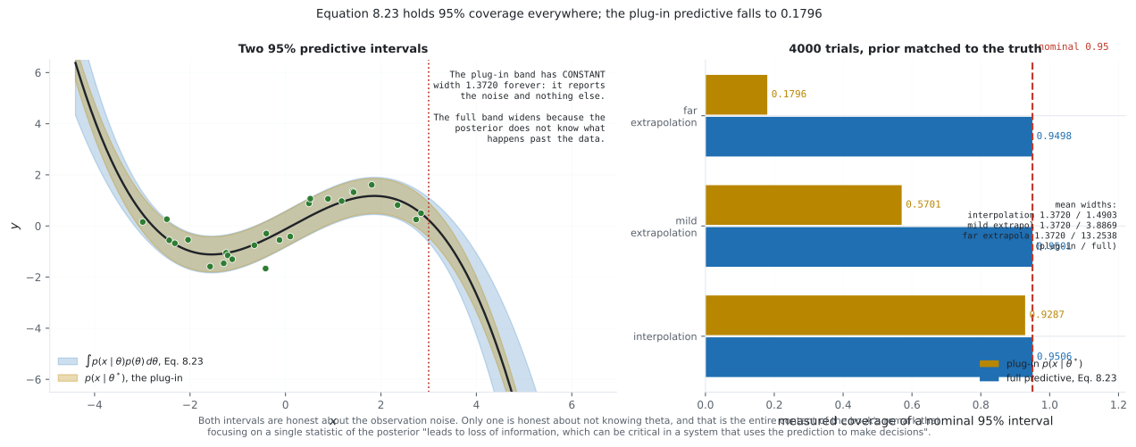
The second figure measures whether that matters, and the answer is unambiguous. The left panel draws both 95% bands. The yellow one has constant width $1.3720$ from one edge of the plot to the other, because $2 \times 1.96 \times \sigma$ contains no reference to $x$. The blue one tracks the data and then flares.

The right panel is the measurement: $4000$ trials with $\boldsymbol\theta$ drawn from the prior and the data drawn from the model — the only setting in which a Bayesian interval is guaranteed calibrated, so the guarantee is what is being tested. It holds: $0.9506$, $0.9501$, $0.9498$. The plug-in interval gives $0.9287$, $0.5701$, $0.1796$. Far from the data it covers the truth 18% of the time while labelled 95% — not a conservative estimate, a wrong one.

This is what the book means by “loss of information, which can be critical in a system that uses the prediction to make decisions.” A system that trusts a 95% label and receives 18% coverage will make confident decisions on inputs it has never seen, and it will be wrong about nineteen times out of twenty-three more often than it was told to expect.

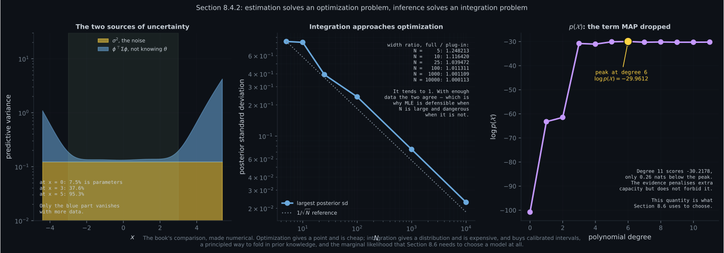
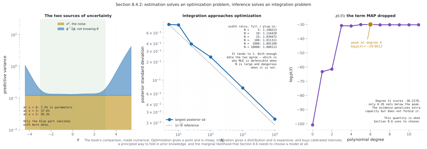
The third figure is the book’s cost-benefit comparison, panel by panel. The left panel splits the predictive variance. The noise floor $\sigma^2 = 0.1225$ is flat — it is a property of the world, and no amount of data removes it. The parameter term $\boldsymbol\phi^\top\boldsymbol\Sigma\boldsymbol\phi$ is $7.5\%$ of the total at $x = 0$ and $95.3\%$ at $x = 5$. Only the second one is reducible, which is the difference between aleatoric and epistemic uncertainty made arithmetic.

The middle panel is why maximum likelihood survives despite everything above. The posterior sd tracks $1/\sqrt{N}$, and the interval-width ratio falls from $1.248213$ at $N = 5$ to $1.000113$ at $N = 10000$. At ten thousand points the two philosophies differ by one part in nine thousand. The expensive machinery earns its cost exactly where data is scarce — which is also exactly where page 803’s overfitting and page 805’s prior mattered most. The chapter keeps arriving at the same boundary.

The right panel is the term MAP dropped. $\log p(\mathcal{X})$ climbs steeply from degree 0 to degree 3 and is then nearly flat, peaking at degree 6. Note the honest reading: degree 11 scores $-30.2178$, only $0.2566$ nats behind the peak — a Bayes factor of $0.7737$, which is not evidence against anything. The marginal likelihood penalises unused capacity automatically, without a validation split and without a tuned $\lambda$, but it penalises it gently. Page 808 is where this becomes a selection rule.

Compare

	maximum likelihood	MAP	Bayesian inference
section	8.3.1	8.3.2	8.4.2
needs a prior	no	yes	yes
needs $p(\mathcal{X})$	no	no, it cancels	yes, and it is an integral
computational problem	optimization	optimization	integration
answer	a point	a point	a distribution
prediction	$p(x \mid \boldsymbol\theta^*)$	$p(x \mid \boldsymbol\theta^*)$	$\int p(x \mid \boldsymbol\theta)p(\boldsymbol\theta)d\boldsymbol\theta$
far-extrapolation coverage	$0.1796$	$0.1796$	$\mathbf{0.9498}$
closed form	often	often	only with a conjugate prior

	parameters $\boldsymbol\theta$	latent variables $\mathbf{z}$
what they do	parametrize the model	describe the generative process
usual treatment	estimated	marginalised out
effect on parameter count	they are the count	often reduces it
in the likelihood	it is a function of them	Eq. 8.25: it must not depend on them
the book’s caveat	—	the separation is “somewhat arbitrary”

pch.quizTag Do you know what integration buys?

1. Section 8.4.1 says a probabilistic model is specified by which object?

   A The likelihood function B The joint distribution of all its random variables C The posterior distribution D The prior distribution
   pch.quizShowAnswer

   B — The joint distribution of all its random variables — Because only the joint has the property that all three of the others follow from it by a rule of probability: the prior and likelihood are its factors by the product rule, the marginal likelihood comes from integrating out the parameters by the sum rule, and the posterior is the joint divided by the marginal. That is why Section 8.5's graphical language describes the joint and nothing else.

2. Measured over 4000 trials with the prior matched to the truth, what coverage does a nominal 95 percent plug-in interval achieve in far extrapolation?

   A 0.9498, the same as the full predictive B 0.1796 — it covers the truth 18 percent of the time while claiming 95 C Exactly 0.95, since the noise model is correct D It is undefined outside the training range
   pch.quizShowAnswer

   B — 0.1796 — it covers the truth 18 percent of the time while claiming 95 — Its width is 1.3720 in every region, because two times 1.96 times sigma contains no reference to x. The full predictive achieves 0.9506, 0.9501 and 0.9498 across the three regions. This is what the book means by loss of information being critical in a system that uses predictions to make decisions.

3. The predictive variance of Equation 8.23 is sigma squared plus phi-transpose Sigma phi. Which part shrinks as you collect more data?

   A Both, at the same rate B Only the second — the noise floor is a property of the world C Only the first D Neither
   pch.quizShowAnswer

   B — Only the second — the noise floor is a property of the world — Measured on the chapter's data, the parameter term is 7.5 percent of the total at x = 0 and 95.3 percent at x = 5. Only that part is reducible. The noise floor of 0.1225 stays whatever you do, which is the difference between uncertainty about the world and uncertainty about your own parameters.

4. The book says estimation and inference differ in their key computational problem. How?

   A Estimation is integration, inference is optimization B Estimation solves an optimization problem; inference solves an integration problem C Both are optimization, at different scales D Both are integration, at different scales
   pch.quizShowAnswer

   B — Estimation solves an optimization problem; inference solves an integration problem — And that is why inference is the expensive one: finding a peak is cheap, summing over everything is not. Measured, the two converge as data accumulates — the interval-width ratio falls from 1.248213 at N = 5 to 1.000113 at N = 10000, which is why maximum likelihood is defensible on large data and reckless on small data.

5. Equation 8.25 marginalises the latent variables out of the likelihood. What does the book insist about the result?

   A That it must still be conditioned on z B That the likelihood must NOT depend on z — only on the data x and the parameters theta C That it only holds for Gaussian latent variables D That it is always analytically tractable
   pch.quizShowAnswer

   B — That the likelihood must NOT depend on z — only on the data x and the parameters theta — Measured on a two-component mixture, the marginal integrates to 1.00000000 in x and mentions z nowhere. That is the point of the two-step procedure: once the latents are integrated out, everything from Sections 8.3 and 8.4.2 applies unchanged, with no new machinery.

6. Everything computed exactly on this page relies on which assumption?

   A That the model class contains the truth B That the prior is conjugate, so the integrals of Equations 8.22 and 8.23 have closed forms C That the data is Gaussian D That N is large
   pch.quizShowAnswer

   B — That the prior is conjugate, so the integrals of Equations 8.22 and 8.23 have closed forms — The book is explicit: without a conjugate prior the integrals are not analytically tractable and you cannot compute the posterior, the predictions, or the marginal likelihood in closed form. Then you need approximations — MCMC, the Laplace approximation, variational inference, or expectation propagation.

Pitfalls

Reporting a plug-in interval as if it were calibrated

Measured across $4000$ trials with the model correct: a nominal $95\%$ plug-in interval achieves $0.9287$ inside the data, $0.5701$ just outside it, and $\mathbf{0.1796}$ far outside. The full predictive achieves $0.9506$, $0.9501$, $0.9498$. The plug-in failure is not conservatism — it is a confident number that is wrong, on exactly the inputs where being wrong is most expensive.

Thinking MAP got the wrong answer

It did not. The posterior mean and the MAP estimate agree to $8.88\times10^{-16}$ for a Gaussian model. The location is identical; what was discarded is the covariance. The criticism of point estimates is about incompleteness, not error.

Expecting Bayesian inference to fix a wrong model class

On the chapter’s own sine data fitted with a cubic, the full predictive reaches only $0.8908$ coverage and the plug-in $0.8580$ — both short of $0.95$. The posterior quantifies uncertainty about $\boldsymbol\theta$ within the model class you chose. It has no way to express “the truth is not a polynomial.” Detecting that is §8.6’s job, not §8.4’s.

Assuming the integrals will be available

Every exact number on this page exists because the prior is conjugate. The book’s warning is that without conjugacy the integrals in Equations 8.22 and 8.23 are “not analytically tractable” and you lose the posterior, the predictions and the marginal likelihood in closed form at once. Budget for MCMC or a variational approximation before committing to a non-conjugate prior.

Paying for integration when N is large

The interval-width ratio is $1.039472$ at $N = 25$ and $1.000113$ at $N = 10000$. Past some sample size the expensive machinery buys a difference smaller than your rounding. The value of a posterior is concentrated exactly where data is scarce, predictions are extrapolations, or decisions are costly.

Treating latent variables as extra parameters

Latent variables “do not parametrize the model explicitly” and usually go with a smaller parameter count, not a larger one — they buy simpler structure and better interpretability. The book also warns that its own split between variables and parameters is “somewhat arbitrary”, since you can always put a prior on a parameter and integrate it out.

Reading the marginal likelihood as a sharp selector

Measured on the chapter’s data: the peak is at degree 6 with $-29.9612$, and degree 11 scores $-30.2178$ — a Bayes factor of $0.7737$, which is no evidence at all. The evidence penalises unused capacity automatically and gently. Treating a $0.26$-nat gap as a decisive verdict reads far more into it than it says.

From the book

This page covers §8.4 of Mathematics for Machine Learning by Deisenroth, Faisal and Ong (draft of 2019-12-11). §8.4.1 is the definition of a probabilistic model as a joint distribution, including the three-way decomposition and the sentence “Only the joint distribution has this property.” §8.4.2 gives Equation 8.22 with the marginal-likelihood integral, Equation 8.23 for the predictive, the margin notes that “Bayesian inference is about learning the distribution of random variables” and that it “inverts the relationship between parameters and the data”, the loss-of-information argument, the optimization-versus-integration comparison, the conjugacy caveat, the list of approximations (MCMC, the Laplace approximation, variational inference, expectation propagation) and of applications, and the remark on the arbitrariness of the variable/parameter split. §8.4.3 gives Equations 8.24 through 8.28, the two-step learning procedure, and the note that the likelihood “must not depend on the latent variables”. §8.4.4 introduces probabilistic programming. The coverage measurements, the variance decomposition, the width-ratio sweep, the marginal-likelihood curve and the mixture verification of Equation 8.25 are this module’s additions.

🧪 Try It Yourself

Exercise 1 – Build the posterior, find the point estimate inside it

pch.exerciseTag pch.exerciseTitle

Exercise 2 – Where the uncertainty comes from

pch.exerciseTag pch.exerciseTitle

Exercise 3 – Does it actually matter?

pch.exerciseTag pch.exerciseTitle

Exercise 4 – The term MAP was allowed to drop

pch.exerciseTag pch.exerciseTitle

Exercise 5 – Integrating out a latent variable

pch.exerciseTag pch.exerciseTitle

Recall card

• Section 8.4.1’s definition: a probabilistic model IS the joint distribution of all its random variables. The prior and likelihood are its factors, the marginal likelihood is what you get by integrating out the parameters, and the posterior is the joint divided by the marginal. Only the joint has that property.
• Equation 8.22 is Bayes’ theorem with the denominator kept. MAP could drop it because it is constant in theta; inference cannot, because it needs the posterior normalised. That integral is the source of every practical difficulty in this section.
• Equation 8.23: the prediction is an average over all plausible parameters, weighted by how plausible each one is. The parameters are marginalised out, so the prediction no longer depends on them at all.
• For a Gaussian model the predictive variance is the noise plus phi-transpose Sigma phi. The mean is identical to the plug-in prediction; only that second term differs, and it is exactly what the point estimate discarded.
• Measured over 4000 trials with the prior matched to the truth: a nominal 95 percent full predictive achieves 0.9506, 0.9501 and 0.9498 across interpolation, mild and far extrapolation. The plug-in achieves 0.9287, 0.5701 and 0.1796.
• The plug-in interval has width 1.3720 in every region, because two times 1.96 times sigma does not depend on where you ask. That constant is the entire failure.
• Only the parameter term is reducible. It is 7.5 percent of the predictive variance at the centre of the data and 95.3 percent two units outside it. The noise floor never goes away.
• The book’s comparison: estimation solves an OPTIMIZATION problem and returns a point; inference solves an INTEGRATION problem and returns a distribution. Predictions from a point are straightforward; predictions from a posterior need another integral.
• They converge. The interval-width ratio falls from 1.248213 at N = 5 to 1.000113 at N = 10000. Maximum likelihood is defensible on large data and reckless on small data, which is the same boundary pages 803 and 805 kept arriving at.
• The posterior mean equals the MAP estimate to 8.88e-16 for a Gaussian. MAP is incomplete, not wrong.
• All of this is exact only because the prior is conjugate. Without conjugacy you lose the posterior, the predictions and the marginal likelihood in closed form simultaneously, and need MCMC, the Laplace approximation, variational inference or expectation propagation.
• Bayesian inference cannot detect a wrong model class. On the chapter’s sine data fitted with a cubic, the full predictive still reaches only 0.8908 coverage. It quantifies doubt about theta inside the class you chose. Choosing the class is Section 8.6.
• Section 8.4.3’s latent variables do not parametrize the model and usually mean fewer parameters, not more. Equation 8.25 integrates them out, and the resulting likelihood must be a function of the data and the parameters only.
• Three posteriors, in order of difficulty: parameters given data, latents given data, both at once — the last is not possible in general. Equation 8.28, the latents given the data AND the parameters, is the tractable compromise, and it is what Chapters 10 and 11 actually compute.
• The marginal likelihood penalises capacity automatically but gently. Measured: the peak is at degree 6, and degree 11 is only 0.2566 nats behind — a Bayes factor of 0.7737, which is no evidence at all.

Next: a picture of the joint distribution, and what you can read off it without doing any algebra. Directed Graphical Models