The Concept of the Margin

Page 1201 ended with $9{,}628$ classifiers that all fit the training data perfectly and disagree on held-out data by $0.1119$. Section 12.2 breaks the tie with one idea: pick the separator that is furthest from the closest point.

The margin is “the distance of the separating hyperplane to the closest examples in the dataset, assuming that the dataset is linearly separable.” Making that precise takes one piece of geometry and one decision.

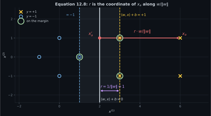
The geometry: r is a coordinate, not a formula

Take a point $\mathbf{x}_a$ and let $\mathbf{x}_a'$ be its orthogonal projection onto the hyperplane. Since $\mathbf{w}$ is normal to the hyperplane — page 1201’s Equation 12.4 — the vector from $\mathbf{x}_a'$ to $\mathbf{x}_a$ points along $\mathbf{w}$, so it is some multiple of the unit vector $\mathbf{w}/\lVert\mathbf{w}\rVert$:

$$\mathbf{x}_a = \mathbf{x}_a' + r\,\frac{\mathbf{w}}{\lVert\mathbf{w}\rVert} \qquad \text{(12.8)}$$

That is all Equation 12.8 says: $r$ is the coordinate of $\mathbf{x}_a$ in the one-dimensional subspace spanned by $\mathbf{w}/\lVert\mathbf{w}\rVert$, measured from the hyperplane. Take the inner product of both sides with $\mathbf{w}$ and add $b$:

$$\langle\mathbf{w}, \mathbf{x}_a\rangle + b = \underbrace{\langle\mathbf{w}, \mathbf{x}_a'\rangle + b}_{=\,0} + \;r\,\frac{\langle\mathbf{w},\mathbf{w}\rangle}{\lVert\mathbf{w}\rVert} = r\lVert\mathbf{w}\rVert$$

so $r = f(\mathbf{x}_a)/\lVert\mathbf{w}\rVert$ — and when $\lVert\mathbf{w}\rVert = 1$, the value of $f$ is the signed distance.

the_projection.py

import numpy as np
 
X = np.array([[3.0,  1.0], [3.0, -1.0], [6.0,  1.0], [6.0, -1.0],
              [1.0,  0.0], [0.0,  1.0], [0.0, -1.0], [-1.0, 0.0]])
Y = np.array([ 1.0,  1.0,  1.0,  1.0,  -1.0, -1.0, -1.0, -1.0])
W_STAR, B_STAR = np.array([1.0, 0.0]), -2.0
 
nw = np.linalg.norm(W_STAR)
R = (X @ W_STAR + B_STAR) / nw               # the signed coordinate
P = X - R[:, None] * (W_STAR / nw)[None, :]  # the projections, via 12.8
 
print(f"{'n':>3} {'x_n':>12} {'r':>8} {'projection':>14} {'distance':>10}")
for n in range(len(X)):
    print(f"{n:>3} {str(X[n]):>12} {R[n]:>8.4f} "
          f"{str(np.round(P[n], 4)):>14} "
          f"{np.linalg.norm(X[n] - P[n]):>10.6f}")
print(f"max |f(x')| over the projections : {np.abs(P @ W_STAR + B_STAR).max():.3e}")
print(f"max | |r| - distance |           : "
      f"{np.abs(np.abs(R) - np.linalg.norm(X - P, axis=1)).max():.3e}")

text

  n          x_n        r     projection   distance
  0      [3. 1.]   1.0000        [2. 1.]   1.000000
  1    [ 3. -1.]   1.0000      [ 2. -1.]   1.000000
  2      [6. 1.]   4.0000        [2. 1.]   4.000000
  3    [ 6. -1.]   4.0000      [ 2. -1.]   4.000000
  4      [1. 0.]  -1.0000        [2. 0.]   1.000000
  5      [0. 1.]  -2.0000        [2. 1.]   2.000000
  6    [ 0. -1.]  -2.0000      [ 2. -1.]   2.000000
  7    [-1.  0.]  -3.0000        [2. 0.]   3.000000
max |f(x')| over the projections : 0.000e+00
max | |r| - distance |           : 0.000e+00

Every projection lands exactly on the hyperplane, and $\lvert r\rvert$ is exactly the distance. The sign carries the side — negative for the four points of the negative class — which is what lets Equation 12.9 fold both classes into one inequality:

$$y_n(\langle\mathbf{w},\mathbf{x}_n\rangle + b) \geq r \qquad \text{(12.9)}$$

figure Equation 12.8: r is the coordinate of x_a along w/||w|| matplotlib

The three green rings are the closest examples. The book's margin note — 'there could be two or more closest examples to a hyperplane' — is the normal case rather than the exception: here three of eight points are tied at distance exactly 1.

With $\lVert\mathbf{w}\rVert = 1$ the margin is just the smallest of those signed values:

the_margin.py

m = Y * (X @ W_STAR + B_STAR)
print(f"y_n f(x_n)  : {m}")
print(f"r = min     : {m.min():.6f}")
print(f"attained at : {list(np.where(np.isclose(m, m.min()))[0])}")

text

y_n f(x_n)  : [1. 1. 4. 4. 1. 2. 2. 3.]
r = min     : 1.000000
attained at : [0, 1, 4]

The decision: a distance needs a scale

Page 1201 measured that $(\mathbf{w}, b)$ and $(c\mathbf{w}, cb)$ are the same classifier for any $c > 0$. So $f(\mathbf{x})$ can be made arbitrarily large without moving anything, and $r$ along with it. The book puts it as a worry about units: “we could change the units of measurement of $\mathbf{x}_n$ and change the values in $\mathbf{x}_n$, and, hence, change the distance to the hyperplane.”

Both halves of that are worth separating, because only one of them is a real hazard.

An isotropic change of units moves the number and not the classifier.

isotropic.py

from scipy.optimize import minimize
 
def hard_margin(XX, YY):
    d = XX.shape[1]
    return minimize(lambda v: 0.5 * v[:d] @ v[:d], np.r_[np.zeros(d) + 0.3, 0.0],
                    constraints=[{"type": "ineq",
                                  "fun": lambda v: YY * (XX @ v[:d] + v[d]) - 1}],
                    method="SLSQP", options={"maxiter": 5000, "ftol": 1e-14})
 
print(f"{'c':>8} {'w after refit':>20} {'margin':>10} {'boundary, orig. coords':>24}")
for c in (0.1, 1.0, 10.0, 100.0):
    r = hard_margin(X * c, Y)
    w, b = r.x[:2], r.x[2]
    print(f"{c:>8.1f} {str(np.round(w, 6)):>20} "
          f"{1/np.linalg.norm(w):>10.4f} {-b/w[0]/c:>24.6f}")

text

       c        w after refit     margin   boundary, orig. coords
     0.1            [10. -0.]     0.1000                 2.000000
     1.0            [ 1. -0.]     1.0000                 2.000000
    10.0            [0.1 0. ]    10.0000                 2.000000
   100.0        [ 0.01 -0.  ]   100.0000                 2.000000

The margin ranges over three orders of magnitude and the decision boundary never moves. A margin of $10$ in millimetres and a margin of $0.01$ in kilometres are the same margin. So the raw value is not comparable across datasets, and Section 12.2’s objective is scale-free in exactly the way it needs to be.

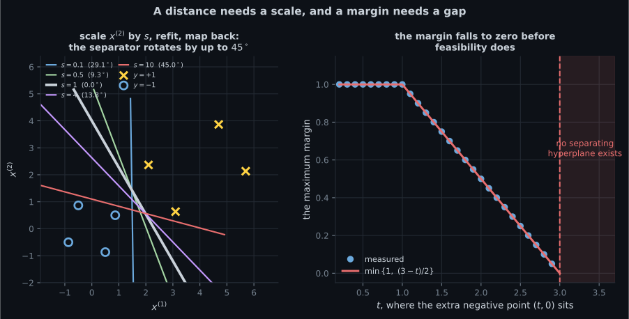
An anisotropic change of units moves the classifier. That one is a genuine modelling decision, and it is Chapter 10’s standardisation question in a new costume. On the running example it happens to do nothing — the separator is already axis-aligned — so the demonstration needs data at an angle:

anisotropic.py

th = np.radians(30.0)
R30 = np.array([[np.cos(th), -np.sin(th)], [np.sin(th), np.cos(th)]])
XR = X @ R30.T                                  # the same data, rotated
 
w0 = hard_margin(XR, Y).x[:2]
w0 = w0 / np.linalg.norm(w0)
 
print(f"{'s on x2':>9} {'unit normal, orig. coords':>28} {'angle moved':>13}")
for s in (0.1, 0.25, 0.5, 1.0, 2.0, 4.0, 10.0):
    r = hard_margin(XR * np.array([1.0, s]), Y)
    wo = np.array([r.x[0], r.x[1] * s])         # map back
    u = wo / np.linalg.norm(wo)
    u = u if u @ w0 >= 0 else -u
    ang = np.degrees(np.arccos(np.clip(u @ w0, -1, 1)))
    print(f"{s:>9.2f} {str(np.round(u, 6)):>28} {ang:>13.6f}")

text

  s on x2    unit normal, orig. coords   angle moved
     0.10          [0.999885 0.015144]     29.132283
     0.25          [0.99555  0.094239]     24.592464
     0.50          [0.935205 0.354108]      9.261223
     1.00          [0.866025 0.5     ]      0.000000
     2.00          [0.866025 0.5     ]      0.000000
     4.00          [0.721254 0.692671]     13.841877
    10.00          [0.258819 0.965926]     45.000000

Forty-five degrees, on data that never moved. Only the units of the second feature changed. At $s = 10$ the fitted normal is $(0.258819, 0.965926)$ — almost perpendicular to the $s = 1$ answer of $(0.866025, 0.5)$. Compare page 1007’s $77.3982^\circ$ from switching height between metres and millimetres: the same phenomenon, and the same conclusion. Standardising is a decision, and the SVM does not make it for you.

figure A distance needs a scale, and a margin needs a gap matplotlib

Right: the measured margins land exactly on min{1, (3-t)/2}. The margin reaches zero at t = 3 and feasibility stops there too — the extra point has entered the rectangle spanned by the positives, so no line can put it outside.

What the margin needs: a gap

Equation 12.10 collects the pieces:

$$\max_{\mathbf{w}, b, r}\ \underbrace{r}_{\text{margin}} \quad\text{subject to}\quad \underbrace{y_n(\langle\mathbf{w},\mathbf{x}_n\rangle + b) \geq r}_{\text{data fitting}}, \quad \underbrace{\lVert\mathbf{w}\rVert = 1}_{\text{normalization}}, \quad r > 0 \qquad \text{(12.10)}$$

The condition $r > 0$ is doing more work than it looks. It requires the data to be linearly separable, and the book flags this in a margin note — “note that $r > 0$ because we assumed linear separability.” Watch it fail:

walking_a_point_in.py

print(f"{'extra negative at':>19} {'separable?':>11} {'margin':>9} {'0.5||w||^2':>12}")
for t in (None, 2.5, 2.9, 3.5, 4.5):
    if t is None:
        XX, YY, name = X, Y, "none"
    else:
        XX, YY, name = np.vstack([X, [t, 0.0]]), np.r_[Y, -1.0], f"({t}, 0)"
    best, bv = None, np.inf
    for s in range(40):                       # many starts: infeasible is real
        rg = np.random.default_rng(s)
        r = minimize(lambda v: 0.5 * v[:2] @ v[:2],
                     np.r_[rg.normal(0, 1, 2), rg.normal(0, 1)],
                     constraints=[{"type": "ineq",
                                   "fun": lambda v: YY * (XX @ v[:2] + v[2]) - 1}],
                     method="SLSQP", options={"maxiter": 5000, "ftol": 1e-14})
        viol = float(np.maximum(0, 1 - YY * (XX @ r.x[:2] + r.x[2])).max())
        if viol < 1e-7 and 0.5 * r.x[:2] @ r.x[:2] < bv:
            bv, best = 0.5 * r.x[:2] @ r.x[:2], r
    if best is None:
        print(f"{name:>19} {'NO':>11} {'--':>9} {'infeasible':>12}")
    else:
        print(f"{name:>19} {'yes':>11} "
              f"{1/np.linalg.norm(best.x[:2]):>9.6f} {bv:>12.6f}")

text

  extra negative at  separable?    margin   0.5||w||^2
               none         yes  1.000000     0.500000
           (2.5, 0)         yes  0.250000     8.000000
           (2.9, 0)         yes  0.050000   200.000000
           (3.5, 0)          NO        --   infeasible
           (4.5, 0)          NO        --   infeasible

The margin collapses continuously; feasibility vanishes abruptly. As the intruding point walks from $2.5$ to $2.9$ the margin falls from $0.25$ to $0.05$ and $\lVert\mathbf{w}\rVert^2$ blows up from $16$ to $400$ — the objective is $1/r^2$, so a vanishing margin is an exploding objective. Then at $t = 3$ the point crosses into the rectangle $[3,6]\times[-1,1]$ spanned by the positive class, and no hyperplane exists at all. Section 12.2.4 is the repair.

Equation 12.10 is not a convex problem

The book presents 12.10 and 12.21 as equivalent, which they are. It does not say that they are equivalent the way a bad formulation is equivalent to a good one.

The constraint $\lVert\mathbf{w}\rVert = 1$ confines $\mathbf{w}$ to a sphere, and a sphere is not a convex set — the midpoint of two unit vectors has norm below $1$. So Equation 12.10 is not a convex program, while Equation 12.21’s feasible set (an intersection of half-spaces) and objective (a quadratic form) are both convex.

Measured over $2{,}000$ random starting points:

formulation	failed to converge	distinct optima found	spread
12.10, $\lVert\mathbf{w}\rVert = 1$	$\mathbf{251}$ — $12.55\%$	$1$	—
12.21, $\min \tfrac12\lVert\mathbf{w}\rVert^2$	$\mathbf{0}$ — $0.00\%$	$1$	$8.9\times10^{-15}$

The non-convexity does not cost accuracy here: every run that converged reached $r = 1$ exactly. It costs reliability — one run in eight simply fails. On a problem this small that is a curiosity; at scale it is the difference between a solver you can trust and one you cannot. Theorem 12.1 is stated as an equivalence, and it is better read as an upgrade.

pch.quizTag Check your understanding

1. A The distance from x_a to the origin B The signed coordinate of x_a along the unit normal, measured from the hyperplane — its absolute value is the distance and its sign says which side C The value of f at x_a, always D The norm of w
   pch.quizShowAnswer

   B — The signed coordinate of x_a along the unit normal, measured from the hyperplane — its absolute value is the distance and its sign says which side

2. A The SVM is broken under rescaling B The classifier changed C The margin has units, so its raw value is not comparable across datasets — but the decision boundary sits in the same place in the original coordinates every time D The data is no longer separable
   pch.quizShowAnswer

   C — The margin has units, so its raw value is not comparable across datasets — but the decision boundary sits in the same place in the original coordinates every time

3. A It standardises the features automatically B Nothing — the relative scaling of features is a modelling decision the method does not make, exactly as in Section 10.6 C It is invariant to it, as the previous table showed D It always picks the axis-aligned solution
   pch.quizShowAnswer

   B — Nothing — the relative scaling of features is a modelling decision the method does not make, exactly as in Section 10.6

4. A The solver runs out of iterations B (3.5, 0) lies inside the rectangle spanned by the positive examples, so no hyperplane can separate it — whereas (2.9, 0) merely squeezes the gap C The margin must be at least 0.1 D The second point is further from the origin
   pch.quizShowAnswer

   B — (3.5, 0) lies inside the rectangle spanned by the positive examples, so no hyperplane can separate it — whereas (2.9, 0) merely squeezes the gap

Exercises

Exercise 1 – Project every point onto the hyperplane

pch.exerciseTag pch.exerciseTitle

Exercise 2 – Walk a point in and watch the margin collapse

pch.exerciseTag pch.exerciseTitle

Exercise 3 – Non-convex against convex, from the same starts

pch.exerciseTag pch.exerciseTitle

Recall card

• The margin is the distance from the hyperplane to the closest example, and Equation 12.8 says that distance is a coordinate: r is where x_a sits along the unit normal, measured from the hyperplane.
• The sign of r carries the side, which is what lets one inequality cover both classes.
• When the norm of w is one, the value of f is the signed distance — so fixing that norm is what turns an arbitrary score into a measurement.
• Ties on the margin are normal, not exceptional. Three of the eight running-example points sit at distance exactly one.
• An isotropic change of units moves the margin and not the classifier. Scaling every feature by 100 takes the margin from 1 to 100 while the boundary stays at exactly the same place.
• An anisotropic change of units moves the classifier. Scaling one feature over two orders of magnitude swings the fitted normal by 45 degrees on data that never moved — Section 10.6’s standardisation decision, in new clothes.
• The condition r greater than zero assumes linear separability, and it is the assumption that fails first on real data.
• The margin collapses continuously but feasibility vanishes abruptly. An intruding point at 2.9 leaves a margin of 0.05 and an objective of 200; at 3.5 there is no separating hyperplane at all.
• Equation 12.10 is not a convex problem, because the unit sphere is not a convex set — measured, a local solver fails on 12.55 percent of random starts.
• Equation 12.21 fails on none of them, and every converged run of either formulation reaches the same answer. Theorem 12.1 is stated as an equivalence and is better read as an upgrade.

Next: Why the Margin Can Be Set to One — §12.2.2 and §12.2.3, the second way to spend the scale, and the proof that the two agree.