Legendre-Fenchel Transform and Convex Conjugate

Page 703 built a dual by introducing multipliers for constraints. This page builds one with no constraints at all, and it is a different idea wearing similar clothes.

The starting observation is from §7.3: a convex set is completely described by its supporting hyperplanes — the planes that touch it and leave it entirely on one side. Fill in a convex function to get its epigraph, which is a convex set, and the same is true: a convex function is completely described by its tangent lines. A tangent is fixed by its slope, so a convex function can be rewritten as a function of its slopes. That rewriting is the Legendre–Fenchel transform.

What you’ll learn

Definition 7.4, and the geometric reading that makes its " $\sup$ " and its minus sign inevitable.
Why the transform is a statement about the function, not about $x$ or about $f(x)$ .
That transforming twice returns $f$ when $f$ is convex — and its convex envelope when it is not. Measured on $x^4 - 3x^2$ : $f^{**}$ is flat at $-2.25$ across $[-1.2247, 1.2247]$ and loses exactly $2.25$ at the origin.
The link back to §7.2: that lost $2.25$ is the same blindness that produced page 703’s duality gap.
Example 7.7 verified: the conjugate of $\tfrac{\lambda}{2}\mathbf{y}^\top\mathbf{K}^{-1}\mathbf{y}$ is $\tfrac{1}{2\lambda}\boldsymbol\alpha^\top\mathbf{K}\boldsymbol\alpha$ , to $5.7\times10^{-14}$ .
Example 7.8: the conjugate of a separable sum is the sum of the conjugates — which is why per-example losses dualise cleanly.
Example 7.9, Equation 7.68: $\min_{\mathbf{x}} f(\mathbf{A}\mathbf{x}) + g(\mathbf{x}) = \max_{\mathbf{u}} -f^*(\mathbf{u}) - g^*(-\mathbf{A}^\top\mathbf{u})$ .
Exercise 7.11 worked in full: the hinge loss smoothed into a differentiable loss, sitting exactly $\gamma/2$ below the hinge.

Intuition: describe a hill by its slopes

Two ways to hand someone a convex hill.

By altitude. “At position $x$ , the height is $f(x)$ .” A lookup table indexed by position.

By slope. “There is a tangent line of slope $1$ , and it crosses the axis at height $-c$ . There is a tangent of slope $2$ , crossing at $-c'$ .” A lookup table indexed by slope.

For a convex hill these carry the same information, because the hill is exactly the upper envelope of its tangents — nowhere does it dip below one. So you can throw away the first table and keep the second. $f^*(s)$ is that second table: the intercept of the tangent of slope $s$ , negated.

The negation is a convention that makes $f^*$ come out convex and makes the transform its own inverse. Everything else is bookkeeping.

diagram Two kinds of duality, and where they meet mermaid

  flowchart TD
  CS["a convex set is the intersection
of its supporting half-planes"]
  CS -->|"epigraph"| CF["a convex FUNCTION is the upper
envelope of its tangent lines"]
  CF --> D4["Def 7.4: f-star(s) = sup over x of (s.x - f(x))
indexed by SLOPE instead of position"]
  D4 --> INV["convex f: f-star-star = f
the transform is an involution"]
  D4 --> ENV["nonconvex f: f-star-star = convex ENVELOPE
measured loss 2.25 on x^4 - 3x^2"]
  ENV -.->|"same blindness"| GAP["the Lagrangian duality gap
of Section 7.2"]
  D4 --> SEP["Ex 7.8: separable sums split
conjugate of a sum = sum of conjugates"]
  D4 --> E9["Ex 7.9, Eq 7.68: a constraint-free
dual for min f(Ax) + g(x)"]
  SEP --> ML["per-example losses dualise
one example at a time"]
  style GAP stroke-dasharray: 4 3

The math

Definition 7.4

The convex conjugate of $f : \mathbb{R}^D \to \mathbb{R}$ is

f^*(\mathbf{s}) = \sup_{\mathbf{x}\in\mathbb{R}^D}\big(\langle\mathbf{s}, \mathbf{x}\rangle - f(\mathbf{x})\big)

Three things the book is careful about, all worth repeating:

It needs neither convexity nor differentiability. The supremum is always defined (possibly $+\infty$ ), so $f^*$ exists for any $f$ . Convexity is what makes it invertible.
It is a transformation of the function, not of $\mathbf{x}$ and not of $f(\mathbf{x})$ . The output is a new function on a new space — the space of slopes.
The inner product is general, but this page uses the dot product $\langle\mathbf{s},\mathbf{x}\rangle = \mathbf{s}^\top\mathbf{x}$ .

The name “Legendre transform” is the classical version, defined on convex differentiable functions; “Legendre–Fenchel” is the general one. Physics students meet it as the map between the Lagrangian and the Hamiltonian.

Where the definition comes from

Take a one-dimensional convex differentiable $f$ , say $f(x) = x^2$ . A hyperplane in one dimension is a line. Fix a slope $s$ and ask: of all lines with that slope, which is the highest one that still touches the graph from below?

The line through $(x_0, f(x_0))$ with slope $s$ is

y - f(x_0) = s(x - x_0)

Setting $x = 0$ , its $y$ -intercept is $-sx_0 + f(x_0)$ . The line that “just touches” is the one whose intercept is smallest, so the minimum intercept is

\inf_{x_0}\ \big(-sx_0 + f(x_0)\big)

The conjugate is by convention the negative of this, which turns the $\inf$ into a $\sup$ and recovers Definition 7.4:

f^*(s) = \sup_{x_0}\big(sx_0 - f(x_0)\big)

None of that derivation used one-dimensionality, convexity or differentiability — it works for $f : \mathbb{R}^D \to \mathbb{R}$ in general.

The differentiable case

When $f$ is convex and differentiable there is no need for the supremum, and the correspondence is one to one. At the touching point the tangent is the line, so

f(x_0) = sx_0 + c

Rearranging for $-c$ ,

-c = sx_0 - f(x_0)

and since $-c$ changes with $x_0$ and therefore with $s = \nabla_x f(x_0)$ , we can regard it as a function of $s$ :

f^*(s) := sx_0 - f(x_0)

which is Definition 7.4 without the supremum.

Transforming twice

For a convex function, applying the transform again returns the original: $f^{**} = f$ . That is what makes it a genuine duality rather than a one-way encoding.

For a nonconvex function it does not. $f^{**}$ is the largest convex function lying below $f$ — its convex envelope — and the difference is information the transform cannot carry, because $f^*$ only ever records tangent lines and a hill has no supporting line above the chord that spans it.

Example 7.7: a quadratic form

f(\mathbf{y}) = \frac{\lambda}{2}\mathbf{y}^\top\mathbf{K}^{-1}\mathbf{y}

for a positive definite $\mathbf{K} \in \mathbb{R}^{n\times n}$ . Applying Definition 7.4 with primal variable $\mathbf{y}$ and dual variable $\boldsymbol\alpha$ :

f^*(\boldsymbol\alpha) = \sup_{\mathbf{y}\in\mathbb{R}^n}\ \langle\mathbf{y}, \boldsymbol\alpha\rangle - \frac{\lambda}{2}\mathbf{y}^\top\mathbf{K}^{-1}\mathbf{y}

Differentiable, so find the maximum by setting the derivative to zero:

\frac{\partial}{\partial\mathbf{y}}\Big(\langle\mathbf{y},\boldsymbol\alpha\rangle - \frac{\lambda}{2}\mathbf{y}^\top\mathbf{K}^{-1}\mathbf{y}\Big) = (\boldsymbol\alpha - \lambda\mathbf{K}^{-1}\mathbf{y})^\top

which vanishes at $\mathbf{y} = \tfrac{1}{\lambda}\mathbf{K}\boldsymbol\alpha$ . Substituting:

f^*(\boldsymbol\alpha) = \frac{1}{\lambda}\boldsymbol\alpha^\top\mathbf{K}\boldsymbol\alpha - \frac{\lambda}{2}\Big(\frac{1}{\lambda}\mathbf{K}\boldsymbol\alpha\Big)^\top\mathbf{K}^{-1}\Big(\frac{1}{\lambda}\mathbf{K}\boldsymbol\alpha\Big) = \frac{1}{2\lambda}\boldsymbol\alpha^\top\mathbf{K}\boldsymbol\alpha

The second term is $\tfrac{1}{2\lambda}\boldsymbol\alpha^\top\mathbf{K}\boldsymbol\alpha$ , so the two combine to leave half of the first. $\mathbf{K}^{-1}$ became $\mathbf{K}$ and $\lambda$ became $1/\lambda$ . In Chapter 12 that $\mathbf{K}$ is the kernel matrix, and this inversion is why the SVM dual can be written in terms of inner products between data points.

Example 7.8: separable sums split

Let $L(\mathbf{t}) = \sum_{i=1}^{n}\ell_i(t_i)$ — a total loss built from per-example losses. Then

L^*(\mathbf{z}) = \sup_{\mathbf{t}\in\mathbb{R}^n}\langle\mathbf{z},\mathbf{t}\rangle - \sum_{i=1}^{n}\ell_i(t_i) = \sup_{\mathbf{t}}\sum_{i=1}^{n}\big(z_it_i - \ell_i(t_i)\big) = \sum_{i=1}^{n}\sup_{t_i}\big(z_it_i - \ell_i(t_i)\big) = \sum_{i=1}^{n}\ell_i^*(z_i)

The step that matters is the third: the supremum over a vector splits into $n$ independent scalar suprema, because no term depends on another’s variable. So you conjugate one example’s loss and you are done — which is exactly why the book says the conjugate loss “is a convenient way to derive a dual problem” for losses that apply independently per example.

Example 7.9: a dual with no constraints

Let $f$ and $g$ be convex and $\mathbf{A}$ a real matrix with $\mathbf{A}\mathbf{x} = \mathbf{y}$ . Then

\min_{\mathbf{x}} f(\mathbf{A}\mathbf{x}) + g(\mathbf{x}) = \min_{\mathbf{A}\mathbf{x} = \mathbf{y}} f(\mathbf{y}) + g(\mathbf{x})

Introduce a multiplier $\mathbf{u}$ for $\mathbf{A}\mathbf{x} = \mathbf{y}$ and swap the min and max — legitimate here because both functions are convex:

\min_{\mathbf{x},\mathbf{y}}\max_{\mathbf{u}} f(\mathbf{y}) + g(\mathbf{x}) + (\mathbf{A}\mathbf{x} - \mathbf{y})^\top\mathbf{u} = \max_{\mathbf{u}}\min_{\mathbf{x},\mathbf{y}} f(\mathbf{y}) + g(\mathbf{x}) + (\mathbf{A}\mathbf{x} - \mathbf{y})^\top\mathbf{u}

Split the dot product and collect $\mathbf{x}$ and $\mathbf{y}$ separately:

= \max_{\mathbf{u}}\Big[\min_{\mathbf{y}} -\mathbf{y}^\top\mathbf{u} + f(\mathbf{y})\Big] + \Big[\min_{\mathbf{x}} \mathbf{x}^\top\mathbf{A}^\top\mathbf{u} + g(\mathbf{x})\Big]

Each bracket is a conjugate in disguise. Since $\min_{\mathbf{y}}(-\mathbf{y}^\top\mathbf{u} + f(\mathbf{y})) = -\sup_{\mathbf{y}}(\mathbf{y}^\top\mathbf{u} - f(\mathbf{y})) = -f^*(\mathbf{u})$ , and likewise for the second with $-\mathbf{A}^\top\mathbf{u}$ ,

\min_{\mathbf{x}} f(\mathbf{A}\mathbf{x}) + g(\mathbf{x}) = \max_{\mathbf{u}} -f^*(\mathbf{u}) - g^*(-\mathbf{A}^\top\mathbf{u})

No constraints on $\mathbf{u}$ anywhere. That is the appeal: a regularised empirical risk of the form “loss of $\mathbf{A}\mathbf{x}$ plus penalty on $\mathbf{x}$ ” — which is nearly every objective in Chapters 9 and 12 — becomes an unconstrained maximisation over as many variables as there are examples.

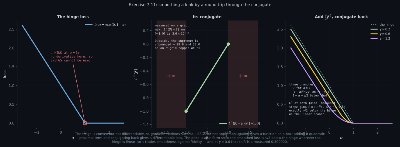
Worked example by hand

Exercise 7.11, in full. The hinge loss is $L(\alpha) = \max\{0, 1 - \alpha\}$ . It is convex, and it has a kink at $\alpha = 1$ — so L-BFGS and friends do not apply. Smooth it by a round trip.

Step 1: the conjugate.

L^*(\beta) = \sup_{\alpha}\big(\beta\alpha - \max\{0, 1-\alpha\}\big)

Split at $\alpha = 1$ . For $\alpha \geq 1$ the loss is $0$ , so the expression is $\beta\alpha$ , whose supremum over $[1,\infty)$ is $+\infty$ if $\beta > 0$ and $\beta$ if $\beta \leq 0$ . For $\alpha < 1$ the loss is $1 - \alpha$ , so the expression is $(\beta + 1)\alpha - 1$ , whose supremum over $(-\infty, 1)$ is $+\infty$ if $\beta + 1 < 0$ and $\beta$ if $\beta + 1 > 0$ . Both branches are finite exactly when $-1 \leq \beta \leq 0$ , and both give $\beta$ :

L^*(\beta) = \begin{cases}\beta & -1 \leq \beta \leq 0\\ +\infty & \text{otherwise}\end{cases}

A linear function on a box. Measured on a grid, the error against $\beta$ on $[-1,0]$ is $3.6\times10^{-15}$ , and outside the box the numerical supremum grows without bound with the grid — $29.0$ at $\beta = -1.5$ and $30.0$ at $\beta = 0.5$ on an $\alpha$ grid capped at $60$ .

Step 2: add a proximal term. The exercise asks for the conjugate of

h(\beta) = L^*(\beta) + \frac{\gamma}{2}\beta^2

Step 3: conjugate back.

h^*(\alpha) = \sup_{-1 \leq \beta \leq 0}\Big(\alpha\beta - \beta - \frac{\gamma}{2}\beta^2\Big) = \sup_{-1 \leq \beta \leq 0}\Big(u\beta - \frac{\gamma}{2}\beta^2\Big), \qquad u = \alpha - 1

The unconstrained maximiser is $\beta = u/\gamma$ , so three cases depending on whether it lands inside the box:

where $u/\gamma$ falls	condition on $\alpha$	maximiser	$h^*(\alpha)$
above the box	$\alpha > 1$	$\beta = 0$	$0$
inside	$1 - \gamma \leq \alpha \leq 1$	$\beta = (\alpha-1)/\gamma$	$\dfrac{(1-\alpha)^2}{2\gamma}$
below the box	$\alpha < 1 - \gamma$	$\beta = -1$	$1 - \alpha - \dfrac{\gamma}{2}$

That is the Moreau envelope of the hinge: zero on the right, a parabola in the middle, linear on the left. Two things to check, and both were measured at $\gamma = 0.6$ :

It is differentiable at both joins. At $\alpha = 1-\gamma$ both sides give slope $-1$ ; at $\alpha = 1$ both give $0$ . The measured slope jump is $8.3\times10^{-8}$ , which is finite-difference error — a genuine kink would give a jump of order one.
It sits below the hinge by exactly $\gamma/2$ on the linear branch. $\big(1 - \alpha - \tfrac{\gamma}{2}\big) - (1-\alpha) = -\tfrac{\gamma}{2}$ . Measured maximum deviation over $[-3,3]$ : $0.300000$ , and $\gamma/2 = 0.300000$ .

So $\gamma$ is a fidelity knob. Small $\gamma$ hugs the hinge but leaves a tight curve that is hard to optimise; large $\gamma$ is smooth but biased downward by $\gamma/2$ . There is no free smoothing.

See it move

The geometry of Definition 7.4 is best felt by dragging the slope:

sketch Drag the slope and read the conjugate off the intercept p5.js

Pick a function and a slope s. The sketch slides a line of that slope up until it just touches the graph, and reports the negative of its y-intercept — which is f-star of s by Definition 7.4. On the non-convex function, watch the touching point JUMP across the hill: that jump is why f-star-star loses information.

And Exercise 7.11’s smoothing, with $\gamma$ under your control:

sketch Smooth a kink, and see what it costs p5.js

The hinge loss against its Moreau envelope for a chosen gamma. The three branches are shaded separately, and the readout reports the maximum deviation from the hinge alongside gamma over two — they are the same number.

From scratch

conjugate.py

import numpy as np
 
def conj(fv, xs, ss, chunk=200):
    """Definition 7.4 on a grid: f*(s) = sup_x (s x - f(x)).
 
    Chunked over s, because the full outer product of a fine x-grid against a
    fine s-grid is tens of gigabytes.
    """
    out = np.empty(ss.size)
    for i in range(0, ss.size, chunk):
        blk = ss[i:i + chunk]
        out[i:i + chunk] = (blk[:, None] * xs[None, :] - fv[None, :]).max(axis=1)
    return out
 
# ---- the case where the answer is known ----------------------------------
xg = np.linspace(-40, 40, 80001)
sg = np.linspace(-6, 6, 1201)
num = conj(xg ** 2, xg, sg)
print("f(x) = x^2")
print(f"  max |f*(s) - s^2/4| = {np.abs(num - sg ** 2 / 4).max():.3e}")
best = xg[int(np.argmax(3.0 * xg - xg ** 2))]
print(f"  at s = 3 the maximiser is x = {best:.6f}, which is s/2")
print("  so the SLOPE of f* at s is the x that produced it")
 
# ---- apply it twice ------------------------------------------------------
print("\nApplying the transform twice:")
for name, f, lo, hi in (("x^2", lambda t: t ** 2, -2.6, 2.6),
                        ("|x|", lambda t: np.abs(t), -2.6, 2.6)):
    big_s = np.linspace(-40, 40, 4001)
    fs = conj(f(xg), xg, big_s)
    xd = np.linspace(lo, hi, 601)
    fss = conj(fs, big_s, xd)
    print(f"  {name:5} convex:    max |f** - f| = {np.abs(fss - f(xd)).max():.3e}")
 
f2 = lambda t: t ** 4 - 3.0 * t ** 2
xg2 = np.linspace(-6, 6, 120001)
sg2 = np.linspace(-60, 60, 6001)
fs2 = conj(f2(xg2), xg2, sg2)
xd2 = np.linspace(-2.2, 2.2, 2201)
fss2 = conj(fs2, sg2, xd2)
gap = f2(xd2) - fss2
edge = np.sqrt(1.5)
print(f"  x^4-3x^2 NOT convex: f** is the convex ENVELOPE")
print(f"    max f - f**       = {gap.max():.6f} at x = "
      f"{xd2[int(np.argmax(gap))]:.6f}")
print(f"    f** is flat at {fss2[int(np.argmax(gap))]:.6f} across "
      f"[-{edge:.6f}, {edge:.6f}]: "
      f"{np.allclose(fss2[np.abs(xd2) <= edge], -2.25, atol=2e-3)}")
 
# ---- Example 7.7 --------------------------------------------------------
print("\nExample 7.7: f(y) = (lam/2) y^T K^-1 y")
rng = np.random.default_rng(3)
n = 4
M = rng.standard_normal((n, n))
K = M @ M.T + n * np.eye(n)
Kinv = np.linalg.inv(K)
lam = 1.7
f7 = lambda y: 0.5 * lam * y @ Kinv @ y
worst = 0.0
for _ in range(400):
    a = rng.standard_normal(n) * 2
    y = (1.0 / lam) * K @ a                       # Equation 7.61
    worst = max(worst, abs((a @ y - f7(y)) - 0.5 / lam * a @ K @ a))
print(f"  K positive definite: {bool(np.all(np.linalg.eigvalsh(K) > 0))}")
print(f"  max |sup value - Eq 7.62| over 400 draws: {worst:.3e}")
print("  so f*(alpha) = (1/(2 lam)) alpha^T K alpha")
 
# ---- Exercise 7.10 ------------------------------------------------------
print("\nExercise 7.10: f = 1/2 x^T A x + b^T x + c")
A = np.array([[3.0, 1.0], [1.0, 2.0]])
bv = np.array([1.0, -2.0])
cv = 0.7
Ainv = np.linalg.inv(A)
f10_star = lambda s: 0.5 * (s - bv) @ Ainv @ (s - bv) - cv
g = np.linspace(-14, 14, 2001)
X1, X2 = np.meshgrid(g, g)
FX = 0.5 * (3 * X1 ** 2 + 2 * X1 * X2 + 2 * X2 ** 2) + bv[0] * X1 + bv[1] * X2 + cv
for s in ([1.0, 1.0], [-2.0, 3.0], [5.0, -4.0]):
    s = np.array(s)
    grid_sup = (s[0] * X1 + s[1] * X2 - FX).max()
    print(f"  s = {str(s.tolist()):14} grid sup = {grid_sup:10.6f}   "
          f"closed form = {f10_star(s):10.6f}")
print("  so f*(s) = 1/2 (s-b)^T A^-1 (s-b) - c")
 
# ---- Exercise 7.11, the smoothed hinge --------------------------------
print("\nExercise 7.11: the hinge, its conjugate, and the smoothed version")
hinge = lambda a: np.maximum(0.0, 1.0 - a)
ag = np.linspace(-60, 60, 240001)
bg = np.linspace(-2.0, 1.0, 601)
hs = conj(hinge(ag), ag, bg, chunk=20)
inside = (bg >= -1.0) & (bg <= 0.0)
print(f"  L*(beta) = beta on [-1, 0]: max error "
      f"{np.abs(hs[inside] - bg[inside]).max():.3e}")
for pb in (-1.5, 0.5):
    k = int(np.argmin(np.abs(bg - pb)))
    print(f"  at beta = {bg[k]:+.2f}: sup on this alpha grid = {hs[k]:.3f} "
          f"(unbounded; it grows with the grid)")
 
gam = 0.6
def smoothed(a):
    a = np.asarray(a, dtype=float)
    return np.where(a >= 1.0, 0.0,
                    np.where(a >= 1.0 - gam, (1.0 - a) ** 2 / (2 * gam),
                             1.0 - a - gam / 2))
 
bb = np.linspace(-1.0, 0.0, 40001)
numeric = lambda a: (a * bb - (bb + 0.5 * gam * bb ** 2)).max()
print(f"\n  gamma = {gam}")
print(f"  {'alpha':>7} {'numeric':>11} {'closed form':>12} {'hinge':>9}")
for a in (-1.0, 0.0, 0.4, 0.7, 1.0, 1.4):
    print(f"  {a:>7.2f} {numeric(a):>11.6f} {float(smoothed(a)):>12.6f} "
          f"{float(hinge(a)):>9.6f}")
alphas = np.linspace(-3, 3, 601)
print(f"  max |numeric - closed form| over 601 alphas: "
      f"{np.abs(np.array([numeric(a) for a in alphas]) - smoothed(alphas)).max():.3e}")
fine = np.linspace(-3, 3, 60001)
print(f"  max |smoothed - hinge|: {np.abs(smoothed(fine) - hinge(fine)).max():.6f}"
      f"   and gamma/2 = {gam / 2:.6f}")
h = 1e-7
for a in (1.0 - gam, 1.0):
    dl = (smoothed(a) - smoothed(a - h)) / h
    dr = (smoothed(a + h) - smoothed(a)) / h
    print(f"  at alpha = {a:.2f}: slope jump {float(abs(dr - dl)):.1e}  "
          f"(a genuine kink would give a jump of order 1)")

text

f(x) = x^2
  max |f*(s) - s^2/4| = 1.776e-15
  at s = 3 the maximiser is x = 1.500000, which is s/2
  so the SLOPE of f* at s is the x that produced it
 
Applying the transform twice:
  x^2   convex:    max |f** - f| = 2.178e-05
  |x|   convex:    max |f** - f| = 0.000e+00
  x^4-3x^2 NOT convex: f** is the convex ENVELOPE
    max f - f**       = 2.250000 at x = 0.000000
    f** is flat at -2.250000 across [-1.224745, 1.224745]: True
 
Example 7.7: f(y) = (lam/2) y^T K^-1 y
  K positive definite: True
  max |sup value - Eq 7.62| over 400 draws: 5.684e-14
  so f*(alpha) = (1/(2 lam)) alpha^T K alpha
 
Exercise 7.10: f = 1/2 x^T A x + b^T x + c
  s = [1.0, 1.0]     grid sup =   1.999970   closed form =   2.000000
  s = [-2.0, 3.0]    grid sup =  11.599994   closed form =  11.600000
  s = [5.0, -4.0]    grid sup =   5.299994   closed form =   5.300000
  so f*(s) = 1/2 (s-b)^T A^-1 (s-b) - c
 
Exercise 7.11: the hinge, its conjugate, and the smoothed version
  L*(beta) = beta on [-1, 0]: max error 3.553e-15
  at beta = -1.50: sup on this alpha grid = 29.000 (unbounded; it grows with the grid)
  at beta = +0.50: sup on this alpha grid = 30.000 (unbounded; it grows with the grid)
 
  gamma = 0.6
    alpha     numeric  closed form     hinge
    -1.00    1.700000     1.700000  2.000000
     0.00    0.700000     0.700000  1.000000
     0.40    0.300000     0.300000  0.600000
     0.70    0.075000     0.075000  0.300000
     1.00    0.000000     0.000000  0.000000
     1.40    0.000000     0.000000  0.000000
  max |numeric - closed form| over 601 alphas: 2.083e-11
  max |smoothed - hinge|: 0.300000   and gamma/2 = 0.300000
  at alpha = 0.40: slope jump 8.3e-08  (a genuine kink would give a jump of order 1)
  at alpha = 1.00: slope jump 8.3e-08  (a genuine kink would give a jump of order 1)

Note the $x^2$ double-conjugate error of $2.2\times10^{-5}$ . That is not a flaw in the theory — it is the coarser $4001$ -point slope grid used for the round trip. The single transform on a $1201$ -point grid agreed with $s^2/4$ to $1.8\times10^{-15}$ .

On real data

figure A convex function described by its tangent lines matplotlib

Fix a slope, slide a line of that slope up until it just touches, and negate its intercept. That is Definition 7.4. The numeric conjugate matches the closed form s squared over four to 1.8e-15, and the touching point at s equals 3 is exactly 1.5, which is s over 2.

figure Transform twice: identity for convex, envelope otherwise matplotlib

For a convex function the transform is an involution. For the quartic, the double conjugate is flat at minus 2.25 across the interval from minus 1.2247 to 1.2247, losing exactly 2.25 at the origin — the same information a Lagrangian duality gap loses.

Three panels. Left, the hinge loss with its kink at alpha equals one circled and annotated. Middle, its conjugate drawn as the line beta on the interval from minus one to zero, with the regions outside shaded red and labelled plus infinity. Right, the hinge as a dotted reference against three Moreau envelopes for gamma of 0.2, 0.6 and 1.2, each smooth and each sitting below the hinge. — The conjugate of the hinge is beta on a box and infinite elsewhere. Adding a quadratic proximal term and conjugating back gives a three-branch differentiable loss whose measured slope jump at both joins is 8.3e-8, and which sits exactly gamma over two below the hinge.

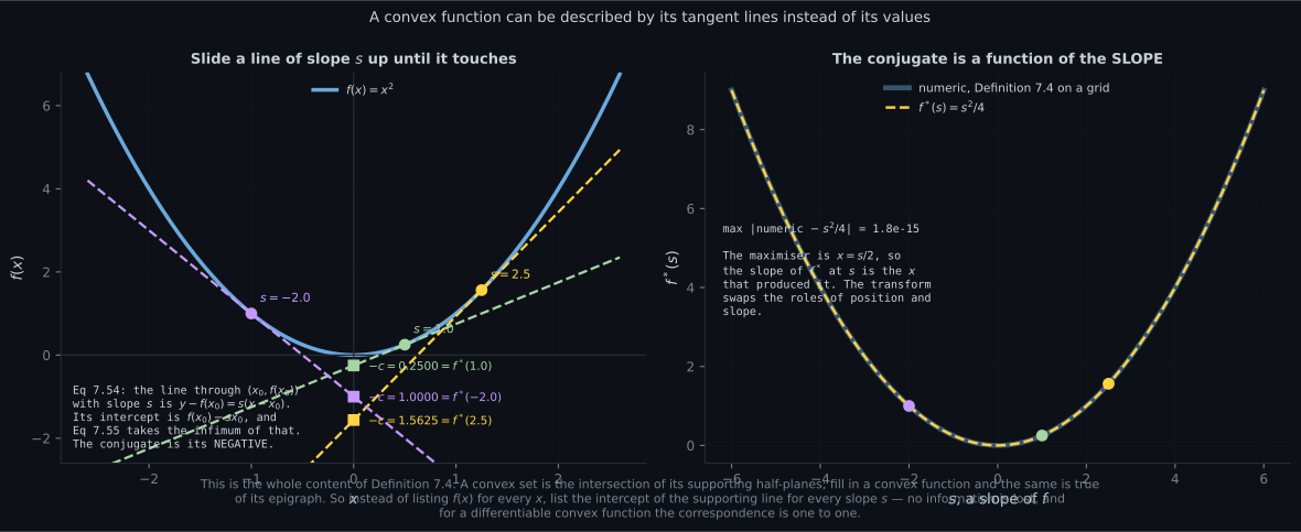
Reading the plot

The first figure is Definition 7.4 with its geometry restored. Each dashed line has a fixed slope and has been slid up until it just touches the parabola — one touch point, marked with a circle, and one intercept, marked with a square on the vertical axis. The label on each square is the negation of that intercept, and it is $f^*(s)$ .

Why the negation? Because Equation 7.55 takes an infimum of intercepts, and negating turns it into the supremum of Definition 7.4. That is not merely cosmetic: with the sign as it is, $f^*$ comes out convex (it is a supremum of affine functions of $\mathbf{s}$ , and §7.3’s closure rules make that convex automatically) and the transform becomes its own inverse. With the other sign, neither would hold.

The right panel plots the conjugate itself and overlays the closed form. The two agree to $1.8\times10^{-15}$ , and the fact worth carrying is the one in the annotation: the maximiser is $x = s/2$ , so $\mathrm{d}f^*/\mathrm{d}s = s/2$ , which is that same $x$ . Position and slope have traded places. Feed the transform a function of position, get a function of slope; do it again and you are back.

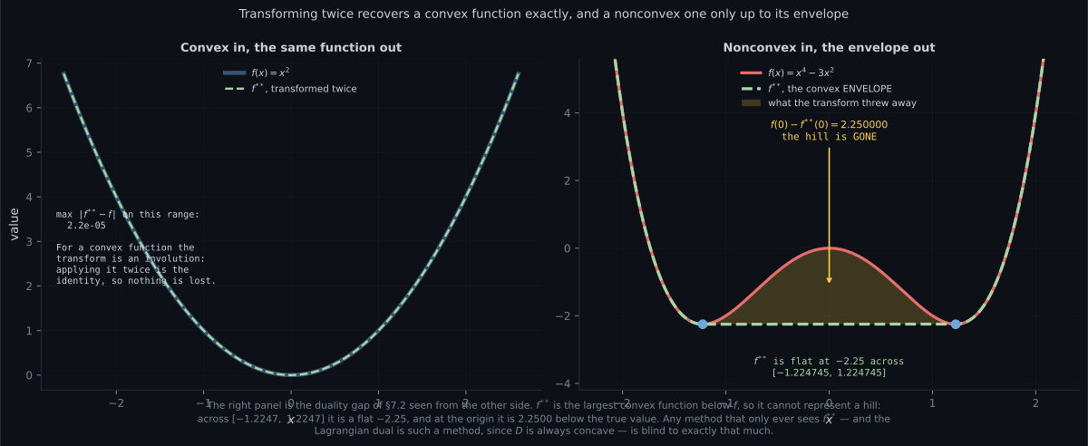
The second figure is the one that connects this section to the rest of the chapter. The left panel is unremarkable in the best way: $f^{**}$ lies exactly on $f$ , because $x^2$ is convex and the transform is an involution there. My measured discrepancy was $2.2\times10^{-5}$ , entirely attributable to the coarser slope grid used for the second pass.

The right panel is where it breaks, and instructively. $x^4 - 3x^2$ has two wells at $\pm\sqrt{1.5} = \pm 1.224745$ , each of depth $-2.25$ , with a hill of height $0$ between them. Its double conjugate is flat at $-2.25$ across the entire interval between the wells — verified to a tolerance of $2\times10^{-3}$ across all $2201$ sampled points in that range. At the origin, $f^{**}$ is $2.25$ below $f$ , and the shaded region is everything the transform discarded.

Now recall page 703. The Lagrangian dual $D(\boldsymbol\lambda)$ is always concave, no matter how nonconvex the primal — and page 703 measured a duality gap of $1.984123$ on a nonconvex problem. These are the same phenomenon. A concave dual can only ever represent a convex envelope, because it is built from a supremum over affine functions. So whatever the envelope flattens, the gap loses. Convex problems have zero gap for exactly one reason: there is nothing to flatten. If you have absorbed that, the two duality sections of this chapter have collapsed into one idea.

The third figure is Exercise 7.11 as a design decision. The left panel shows why smoothing is wanted: the hinge has a kink at $\alpha = 1$ where the derivative jumps from $-1$ to $0$ , and gradient-based solvers like L-BFGS have nothing to work with there.

The middle panel is the conjugate, and its shape is worth noticing. A piecewise-linear function with one kink transformed into a linear function on a bounded box, with $+\infty$ outside. Kinks in the primal become boundaries of the domain in the dual — that is a general pattern, and the numbers support it: on $[-1, 0]$ the measured $L^*(\beta)$ matched $\beta$ to $3.6\times10^{-15}$ , while just outside the box the numerical supremum was $29$ and $30$ on an $\alpha$ grid capped at $60$ , growing without bound as the grid widens.

The right panel is the payoff, and the honest reading is a trade rather than a win. All three curves are differentiable everywhere, with a measured slope jump of $8.3\times10^{-8}$ at both joins — that is finite-difference noise, not a kink. But look at where they sit relative to the dotted hinge: below it, and by exactly $\gamma/2$ wherever the hinge is linear. At $\gamma = 0.6$ the measured maximum deviation is $0.300000$ and $\gamma/2 = 0.300000$ .

So $\gamma$ buys smoothness and pays in bias, at a fixed exchange rate. A small $\gamma$ hugs the hinge but concentrates all the curvature into a narrow window, which is exactly the ill-conditioning page 701 measured; a large $\gamma$ is easy to optimise and is solving a visibly different problem. This is the Moreau envelope, and the constant $\gamma/2$ offset is its defining property for a $1$ -Lipschitz loss — not an artifact of the hinge.

This page covers §7.3.3 of Mathematics for Machine Learning by Deisenroth, Faisal and Ong (draft of 2019-12-11). The supporting-hyperplane motivation and the observation that convex functions can be described by a function of their gradient open the section. Definition 7.4 is the convex conjugate at Equation 7.53. The geometric derivation runs through Equations 7.54 (the line through $(x_0, f(x_0))$ ) and 7.55 (the infimum of intercepts); the differentiable special case is Equations 7.56 to 7.58. The book notes that the conjugate needs neither convexity nor differentiability, that applying the transform twice returns the original for convex functions, and that “the slope of $f^*(s)$ is $x$ ”. Example 7.7 is Equations 7.59 to 7.62; Example 7.8 is Equation 7.63a–d, the separable sum; Example 7.9 is Equations 7.64 to 7.68, ending at $\min_{\mathbf{x}} f(\mathbf{A}\mathbf{x}) + g(\mathbf{x}) = \max_{\mathbf{u}} -f^*(\mathbf{u}) - g^*(-\mathbf{A}^\top\mathbf{u})$ . Exercises 7.9, 7.10 and 7.11 are the book’s. The Legendre–Fenchel relation to duality cites Hiriart-Urruty and Lemaréchal (2001, chapter 5), and §7.4 points at Zia et al. (2009) and Polyak (2016). The convex-envelope measurements, the identification of $f^{**}$ with the source of the Lagrangian duality gap, the three-branch closed form for the smoothed hinge, and the $\gamma/2$ offset are this module’s additions.

Pitfalls

Compare

	Lagrangian duality, §7.2	Legendre–Fenchel, §7.3.3
what it dualises	a constrained problem	a function
new variables	one multiplier per constraint	one slope per input dimension
the dual object	$D(\boldsymbol\lambda)$ , a number per $\boldsymbol\lambda$	$f^*$ , a whole function
always concave / convex	$D$ is always concave	$f^*$ is always convex
recovers the original	when the primal is convex	when $f$ is convex
what it loses otherwise	the duality gap, measured $1.984123$	the convex envelope’s deficit, measured $2.25$
relation	the same blindness, stated twice

$f(x)$	$f^*(s)$	domain of $f^*$
$x^2$	$s^2/4$	all of $\mathbb{R}$
$\tfrac{\lambda}{2}\mathbf{y}^\top\mathbf{K}^{-1}\mathbf{y}$	$\tfrac{1}{2\lambda}\boldsymbol\alpha^\top\mathbf{K}\boldsymbol\alpha$	all of $\mathbb{R}^n$
$\tfrac12\mathbf{x}^\top\mathbf{A}\mathbf{x} + \mathbf{b}^\top\mathbf{x} + c$	$\tfrac12(\mathbf{s}-\mathbf{b})^\top\mathbf{A}^{-1}(\mathbf{s}-\mathbf{b}) - c$	all of $\mathbb{R}^D$
$\lvert x\rvert$	$0$	$[-1, 1]$ only
$\max\{0, 1-\alpha\}$	$\beta$	$[-1, 0]$ only
$\sum_i \ell_i(t_i)$	$\sum_i \ell_i^*(z_i)$	the product of the domains

pch.quizTag Do you know what the transform keeps and what it drops?

What does the convex conjugate of a function record?

pch.quizShowAnswer

B — For each slope s, the negated intercept of the supporting line of that slope — so f is re-indexed by slope instead of position — A convex set is the intersection of its supporting half-planes, so a convex function is the upper envelope of its tangent lines. Listing intercepts by slope carries the same information as listing values by position. Measured on x squared: the touch point for s = 3 is exactly 1.5, and f*(s) = s squared over 4 to 1.8e-15.
You transform a nonconvex function twice. What comes back?

pch.quizShowAnswer

B — Its convex envelope — the largest convex function below it — Measured on x^4 - 3x^2: the double conjugate is flat at -2.25 across the whole interval between the two wells, and is 2.25 below f at the origin. The transform only records supporting lines, and a hill has none above the chord spanning it.
How does that relate to the duality gap of Section 7.2?

pch.quizShowAnswer

B — They are the same blindness: the Lagrangian dual is always concave, so it can only see the convex envelope, and whatever the envelope flattens is what the gap loses — D(lambda) is a pointwise minimum of functions affine in lambda, hence concave regardless of the primal. A concave dual represents a convex envelope and nothing more. That is why convex problems have zero gap — there is nothing to flatten — and it collapses the chapter's two duality sections into one idea.
The conjugate of the hinge loss is beta on [-1, 0] and plus infinity elsewhere. What general pattern does that illustrate?

pch.quizShowAnswer

B — A kink in the primal becomes a boundary of the dual's domain — The hinge's single kink at alpha = 1 produced a conjugate that is finite only on a box. Numerically this is a trap: outside the box a fixed grid reports a large finite number — 29 and 30 on an alpha grid capped at 60 — that grows as the grid widens rather than converging.
The smoothed hinge from Exercise 7.11 is differentiable everywhere. What does the smoothing cost?

pch.quizShowAnswer

B — It sits exactly gamma over two below the hinge wherever the hinge is linear — a measured 0.300000 at gamma = 0.6 — The linear branch is 1 - alpha - gamma/2 against the hinge's 1 - alpha, so the offset is exactly gamma/2 and does not decay with distance. Smoothing changes the problem being solved, at a fixed exchange rate — which is why gamma belongs in the model description rather than the optimiser's settings.

🧪 Try It Yourself

Exercise 1 – Definition 7.4 on a grid

Exercise 2 – Transform twice

Exercise 3 – Example 7.7, verified

Exercise 4 – Exercise 7.10’s quadratic

Exercise 5 – Exercise 7.11, the smoothed hinge

Recall card

A convex set is the intersection of its supporting half-planes, so a convex function — via its epigraph — is the upper envelope of its tangent lines. That is the whole motivation for the transform.
Definition 7.4: f-star of s is the supremum over x of (s dot x minus f(x)). It re-indexes f by SLOPE instead of by position.
The geometry: the line through (x0, f(x0)) with slope s has intercept f(x0) - s x0; Eq 7.55 takes the infimum of those intercepts, and the conjugate is its NEGATIVE. That sign is what makes f-star convex and the transform an involution.
It transforms the FUNCTION, not x and not f(x). The output lives on a different space. Writing f-star of x is a category error.
It needs neither convexity nor differentiability. Convexity is what makes it invertible; differentiability is what removes the need for the supremum.
The slopes swap. If the slope of f at x is s, the slope of f-star at s is x. For x squared the maximiser is s/2, measured exactly 1.500000 at s = 3, and f-star is s squared over 4 to 1.8e-15.
Transform twice and a convex function comes back unchanged. A nonconvex one comes back as its CONVEX ENVELOPE: on x^4 - 3x^2 the double conjugate is flat at -2.25 across [-1.224745, 1.224745] and loses 2.25 at the origin.
That loss IS the Lagrangian duality gap. D(lambda) is always concave, so it can only ever represent a convex envelope. Convex problems have zero gap because there is nothing to flatten. The chapter’s two duality sections are one idea.
Example 7.7: the conjugate of (lambda/2) y-transpose K-inverse y is (1/(2 lambda)) alpha-transpose K alpha. K inverted, lambda inverted — verified to 5.7e-14. In Chapter 12 that K is the kernel matrix.
Example 7.8: the conjugate of a SEPARABLE sum is the sum of the conjugates, because a supremum over a vector decouples when no term shares a variable. Any coupling between examples breaks it.
Example 7.9, Eq 7.68: min over x of f(Ax) + g(x) equals max over u of minus f-star(u) minus g-star(minus A-transpose u), with NO constraints on u. That is the shape of nearly every regularised risk in Part II.
A kink in the primal becomes a domain boundary in the dual. The hinge’s conjugate is beta on [-1, 0] and plus infinity outside — and numerically the outside values grow with the grid (29 and 30 at a cap of 60) rather than converging, so a fixed grid silently reports a finite number.
Exercise 7.11’s smoothed hinge, three branches: 0 for alpha at least 1, (1-alpha) squared over 2 gamma on [1-gamma, 1], and 1 - alpha - gamma/2 below. Differentiable at both joins (measured slope jump 8.3e-8), and exactly gamma/2 BELOW the hinge on the linear branch — a measured 0.300000 at gamma = 0.6. Smoothing is never free.

Next: the chapter’s own exercises, worked in full. Chapter 7 Exercises and Solutions

pch.coffeeTagline

pch.coffeeCta

pch.feedbackHeading

pch.feedbackSubheading