Phase 4 - Sequence Models with RNNs

Everything before this phase assumed a fixed-size input. Sequences break that twice over: their order carries meaning, and their length varies. A recurrent layer handles both by walking the sequence one element at a time and carrying a state forward — so its parameter count is independent of length (SimpleRNN(32) is 2,080 parameters for 20 timesteps or 20,000).

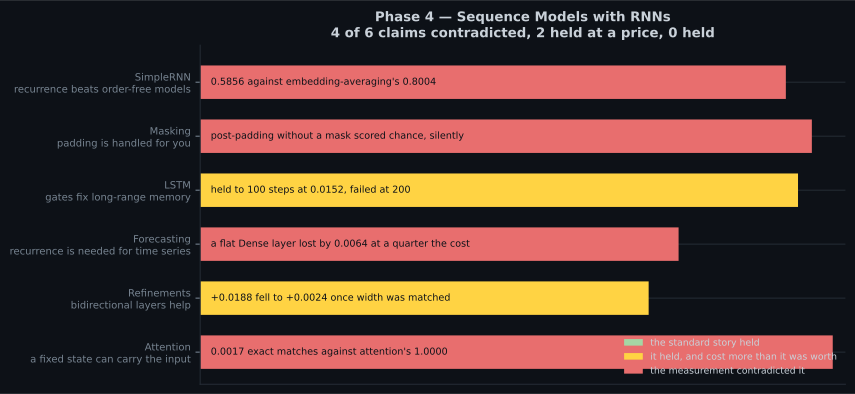
The measurements in this phase are unusually blunt about what that buys. On 5,000 IMDB reviews, a SimpleRNN(32) scored 0.5856 while averaging the same embeddings and throwing away order entirely scored 0.8004. Gated cells then took it to 0.8156. Sequence modelling is a story about a mechanism that does not work until it is fixed twice.

The pages

#	Page	The measured headline
431	Intro to RNNs	the cell in five lines of NumPy, matching Keras at 2.68e-07; order is worth +0.0744 to the RNN and +0.0000 to a bag of words — which still won
431.5	Padding, Masking and Variable-Length Sequences	post-padding without a mask scores 0.5036 — chance — with no error and a falling loss curve
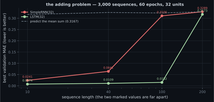
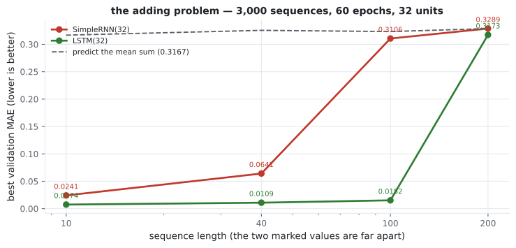
432	LSTM & GRU Networks	gates re-derived in NumPy to 6.56e-07; +0.23 accuracy over a SimpleRNN, and at 80 steps MAE 0.0056 against 0.2984
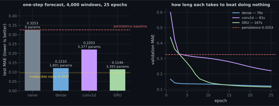
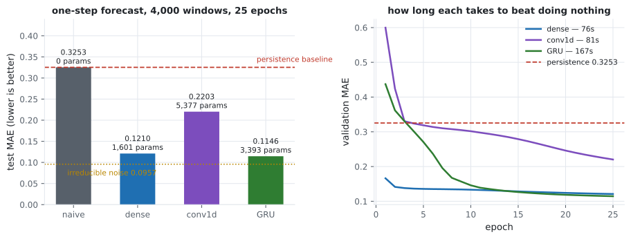
433	Time Series Forecasting	persistence 0.3253, noise floor 0.0965, Dense 0.1210 against GRU 0.1146 at a quarter of the cost
434	Advanced Recurrent Layers	of three refinements only dropout helped (+0.0104); recurrent_dropout cost 2.0× the wall-clock to lose 0.0080; stacking lost at every depth; Bidirectional’s +0.0188 fell to +0.0024 at matched width
434.5	Attention Before Transformers	the fixed-state bottleneck, measured: 0.0017 exact matches against 1.0000, and a per-position split showing the year at 1.0000 and the day’s last digit at 0.0908

diagram Diagram mermaid

  flowchart TD
  A["431 The recurrence
h_t = tanh(Wx·x + Wh·h + b)"] --> B["431.5 Padding & masking
pre/post, mask_zero"]
  B --> C["432 Gated cells
LSTM, GRU"]
  C --> D["433 Forecasting
windows, baselines, horizons"]
  C --> E["434 Refinements
dropout, stacking, bidirectional"]
  C --> G["434.5 Additive attention
the bottleneck, removed"]
  D --> F["Phase 5: attention
replaces recurrence"]
  E --> F
  G --> F

figure The adding problem — 3,000 sequences, 60 epochs, 32 units matplotlib

The SimpleRNN solves the task at 10 and 40 steps, then collapses onto the baseline at 100: it has not merely got worse, it has stopped carrying the number at all. The LSTM holds to 100 steps at MAE 0.0152 — twenty times better — and then fails too at 200. That last column is honest rather than convenient: the gates raise the length at which recurrence works, they do not make it unbounded, and 60 epochs is a modest budget for a 200-step credit assignment.

figure One-step forecast: 4,000 windows, 25 epochs matplotlib

The GRU wins by 0.0064 over a flattened Dense layer while costing 4.3x the wall-clock and twice the parameters — and both sit close to the 0.0965 noise floor, so there was very little left to win. The Conv1D stack is the interesting failure: 5,377 parameters, still improving at epoch 25, and beaten by a single Dense layer. Its two pooling and convolution stages blur exactly the recent detail a one-step forecast depends on.

figure Every claim this phase set out to test matplotlib

Collected from the runs behind each page's own figures rather than measured afresh, so every bar is traceable to the page it names. Bar length is the log of the effect size, because the effects span from 0.0014 to 5,376 — the number that matters is printed on each bar. Across all nine phases, 34 of 54 claims were contradicted outright, 11 held at a cost that was worth stating, and 9 held as advertised.

Three things this phase measures that most treatments assert

1. A SimpleRNN is not a working sequence model at 200 timesteps. It lost to embedding-averaging by 0.2148. The gap is not a tuning failure — it is the vanishing-signal problem that gated cells were invented for, and the phase measures it before fixing it.
2. The padding bug is silent. Identical code with padding="post" and no mask converged smoothly to 0.5036 on a balanced binary task. Nothing warns you; the loss curve looks healthy; only the accuracy tells you, and only if you know what chance is.
3. A flattened Dense layer is a serious forecasting baseline. It scored 0.1210 against the GRU’s 0.1146 in a quarter of the wall-clock, with the irreducible noise floor at 0.0965. Recurrence pays when the useful information is far back and order-dependent — not merely because the data has a time axis.

sketch How far back can it remember? p5.js Pause Restart

Drag the slider to set the sequence length. The bars are measured MAE on the adding problem for a SimpleRNN and an LSTM, against the do-nothing baseline.

The habit this phase is really teaching

Every page here compares against something that costs nothing:

Task	The do-nothing baseline	What it exposed
sentiment	average the embeddings (0.8004)	the SimpleRNN was not working
masking	chance on a balanced task (0.5000)	post-padding scored 0.5036
long-range recall	predict the mean sum (0.3324)	the SimpleRNN reached 0.2984 — a tenth of the way — while the GRU reached 0.0056
forecasting	persistence (0.3253), noise floor (0.0965)	the GRU’s win over Dense was 0.0064
date normalisation	the same model without attention (0.0017)	attention reached 1.0000 exact match

A sequence model that has not been compared against one of these has not been measured. That is why the same discipline reappears in Phase 5, where the baseline for a transformer is often a bag of words, and in Phase 6, where the baseline for a generative model is the training data itself.

sketch How often the standard story survived p5.js Pause Restart

Step through the phases. Each bar splits the claims that phase tested into contradicted, held at a price, and held as advertised - the totals are summed live.

What carries forward

Idea from this phase	Where it comes back
padding, masks, and which layers honour them	attention masks in every transformer
additive state updates under a gate	residual streams, gated MLPs
return_sequences and per-timestep outputs	seq2seq decoders, per-token losses
layer normalisation over features, not batch	every transformer block
chronological splits and leakage	any temporal evaluation, including RL

From the book

Hands-On Machine Learning frames an RNN as a chain that can be unrolled into a very deep feedforward network — one copy per timestep, all sharing weights — and trained with backpropagation through time. Page 431 makes that literal: the five-line NumPy loop is the layer, matched against Keras to 2.68e-07, and the 200-step state trace shows what “very deep” costs when 132 of those steps are padding.

From the book

Chollet’s advice on sequences is to start with a common-sense baseline and only then add machinery. Page 433 takes that seriously enough to compute the irreducible error: with noise of $\sigma = 0.12$, no forecaster can beat MAE $\sigma\sqrt{2/\pi} = 0.0958$, and the best model here reached 0.1146. Knowing that number is the difference between “tune further” and “stop”.

pch.quizTag pch.quizDefaultTitle

1. A `SimpleRNN(32)` scored 0.5856 on IMDB while averaging the same embeddings - discarding order entirely - scored 0.8004. What does the gap show?

   A That word order is irrelevant to sentiment B That the SimpleRNN is not functioning as a sequence model at 200 timesteps: it is losing signal across the chain faster than it gains from order C That the embeddings were badly initialised D That the baseline was computed incorrectly
   pch.quizShowAnswer

   B — That the SimpleRNN is not functioning as a sequence model at 200 timesteps: it is losing signal across the chain faster than it gains from order

2. Identical code with `padding="post"` and no mask converged smoothly to 0.5036 on a balanced binary task. Why is this the most dangerous bug in the phase?

   A Because it crashes at inference time B Because nothing signals it - no error, no warning, and a healthy-looking falling loss curve - so it is only visible if you know what chance-level accuracy is for your task C Because it corrupts the training data D Because it only happens with LSTMs
   pch.quizShowAnswer

   B — Because nothing signals it - no error, no warning, and a healthy-looking falling loss curve - so it is only visible if you know what chance-level accuracy is for your task

3. A flattened `Dense` layer scored 0.1210 on forecasting against the GRU's 0.1146, with the irreducible noise floor at 0.0965. What does the noise floor add?

   A Nothing - only the model comparison matters B It converts a 0.0064 gap into a judgement: both models are close to the best achievable score, so there is very little left to win and 4.3x the wall-clock buys almost none of it C It proves the GRU is overfitting D It sets the learning rate
   pch.quizShowAnswer

   B — It converts a 0.0064 gap into a judgement: both models are close to the best achievable score, so there is very little left to win and 4.3x the wall-clock buys almost none of it

4. Of three refinements, `recurrent_dropout` cost 2.0x the wall clock to LOSE 0.0080, and `Bidirectional`'s +0.0188 fell to +0.0024 once width was matched. What does the width-matching change?

   A Nothing, it is a formality B A bidirectional layer doubles the parameters, so the naive comparison credits attention-to-both-directions for a gain that is mostly extra capacity C It makes the model slower D It changes the masking behaviour
   pch.quizShowAnswer

   B — A bidirectional layer doubles the parameters, so the naive comparison credits attention-to-both-directions for a gain that is mostly extra capacity

5. The LSTM held MAE 0.0152 at 100 timesteps but failed at 200, landing on the do-nothing baseline. Why report the failure column?

   A To fill out the table B Because it bounds the claim: gates raise the length at which recurrence works rather than removing the limit, and the reader needs to know where the limit sits C Because the LSTM was broken D Because 200 steps is unrealistic
   pch.quizShowAnswer

   B — Because it bounds the claim: gates raise the length at which recurrence works rather than removing the limit, and the reader needs to know where the limit sits