Discrete and Continuous Probabilities

§6.1 built one distribution, on a target space with three elements. This section asks what changes when the target space is not a short list — and the answer is more than bookkeeping. The object that describes a continuous random variable is not a probability, and reading it as one is the single most common error in this chapter.

The book is unusually blunt about the notation:

Unfortunately, machine learning literature uses notation and nomenclature that hides the distinction between the sample space $\Omega$, the target space $\mathcal{T}$, and the random variable $X$.

Table 6.1 exists to undo that, and it is reproduced below.

What you’ll learn

• pmf, pdf, cdf — three different objects, and which of them is ever a probability.
• Definition 6.1: a pdf is any non-negative function that integrates to one. Note what is not required.
• Why a density of $39.9$ is completely normal, and why $P(X = x) = 0$ for a continuous random variable.
• Definition 6.2 and Equation 6.18: the cdf, and the cdf as the integral of the pdf.
• Example 6.2 in full: the joint of Equation 6.9, the marginals of 6.10 and 6.11, and both conditionals, 6.13 and 6.14 — including which axis ends up summing to one.
• Example 6.3, the pair of uniform distributions the book uses to make the height point, with Equation 6.19 checked.
• Table 6.1’s nomenclature, and the Remark that discrete states need not have an order.

Intuition: a bar chart and a rope

A pmf is a bar chart. Each bar is the probability of one state, so each bar is between $0$ and $1$, and the bars add to $1$. Nothing surprising happens.

A pdf is a rope of fixed total length laid over an interval. The area under it is $1$ — always — but the height is whatever it needs to be to make that true. Squeeze the rope onto a narrow interval and it piles up: the same unit of area over a width of $0.01$ has to reach a height of $100$. There is no rule against that, because the height was never a probability.

The pmf answers “how likely is this state?” The pdf answers nothing on its own; you have to integrate it over an interval before it answers anything. And the question “how likely is exactly $x$?” has the answer zero in the continuous case — not “very small”, exactly zero, because an interval of zero width has zero area.

The cdf is the accumulated area from the left. It runs from $0$ to $1$, never exceeds either, and is a probability at every single point. If you only remember one of the three as “the safe one”, remember the cdf.

diagram Diagram mermaid

  flowchart TD
  T{"is the target space
discrete or continuous?"}
  T -->|"discrete"| PMF["pmf: P(X = x)
Eq 6.12"]
  T -->|"continuous"| PDF["pdf: p(x)
Definition 6.1"]
  PMF --> PB["each value is a PROBABILITY
so each is at most 1"]
  PDF --> PD["each value is a DENSITY
unbounded above"]
  PDF --> Z["P(X = x) = 0 exactly
an interval of zero width"]
  PDF --> INT["integrate over [a, b]
Eq 6.16 -> a probability"]
  PMF --> CDF["cdf: P(X <= x)
Definition 6.2"]
  INT --> CDF
  CDF --> SAFE["always in [0, 1]
the only one always a probability"]
  PMF -.->|"Section 6.3"| J["joint, marginal, conditional"]
  PDF -.->|"Section 6.7"| CV["change of variables
needs the Jacobian"]

The math

Which object goes with which target space

When $\mathcal{T}$ is discrete, you can name the probability that $X$ takes a particular value, $P(X = x)$. That expression is the probability mass function.

When $\mathcal{T}$ is continuous — say the real line — it is more natural to give the probability that $X$ lands in an interval, $P(a \leqslant X \leqslant b)$. By convention one specifies $P(X \leqslant x)$, and that expression is the cumulative distribution function.

The book also fixes two words used throughout: univariate for a single random variable (states written non-bold, $x$) and multivariate for several, usually a vector of random variables (states bold, $\mathbf{x}$).

6.2.1 Discrete: a table of numbers

With a discrete target space you can picture the distribution of several random variables as filling in a multidimensional array. The target space of the joint is the Cartesian product of the individual target spaces, and the joint probability is one entry of the array:

$$P(X = x_i, Y = y_j) = \frac{n_{ij}}{N} \tag{6.9}$$

where $n_{ij}$ is the number of events with state $x_i$ and $y_j$, and $N$ the total. This is the probability of an intersection: $P(X = x_i, Y = y_j) = P(X = x_i \cap Y = y_j)$.

Three names go with three operations on that table, and they are all just different divisors:

• the joint $p(x, y)$ — a cell over the grand total;
• the marginal $p(x)$ — a row or column total over the grand total, “the probability that $X = x$ irrespective of $Y$”;
• the conditional $p(y \mid x)$ — a cell over a row or column total.

The notation $X \sim p(x)$ means ”$X$ is distributed according to $p(x)$”.

6.2.2 Continuous: densities

The book is candid that it treats real random variables as though they were discrete with finitely many states, and flags the two places that breaks: when something is repeated infinitely often (Chapter 8’s generalisation error), and when drawing a point from an interval.

The technicality, stated once

Two things go wrong in continuous spaces. First, the set of all subsets is not well behaved — $\mathcal{A}$ has to be restricted so it survives complements, intersections and unions. Second, the size of a set is subtle: cardinality for discrete sets, length for an interval of $\mathbb{R}$, volume in $\mathbb{R}^d$ are all measures. Sets that behave under set operations and carry a topology form a Borel σ-algebra, and that is what the book assumes for real-valued random variables. This is the same problem §6.1’s power set ran into, and the σ-algebra is the fix.

Definition 6.1 (Probability Density Function). A function $f : \mathbb{R}^D \to \mathbb{R}$ is a pdf if

1. $\forall \mathbf{x} \in \mathbb{R}^D : f(\mathbf{x}) \geqslant 0$
2. its integral exists and

$$\int_{\mathbb{R}^D} f(\mathbf{x})\,\mathrm{d}\mathbf{x} = 1 \tag{6.15}$$

Read the definition again and notice what is absent: no upper bound on $f(\mathbf{x})$. Non-negative, integrates to one. That is the entire requirement. For a pmf, the integral in 6.15 becomes the sum in 6.12.

A random variable $X$ is associated with $f$ by

$$P(a \leqslant X \leqslant b) = \int_a^b f(x)\,\mathrm{d}x \tag{6.16}$$

and that association is the law or distribution of $X$.

The Remark that follows Equation 6.16

For a continuous random variable, $P(X = x) = 0$. The book’s one-line reason is the best one: it is Equation 6.16 with $a = b$ — an integral over an interval of zero width. In the margin: ”$P(X = x)$ is a set of measure zero.”

Definition 6.2 (Cumulative Distribution Function). For a multivariate real-valued $X$ with states $\mathbf{x} \in \mathbb{R}^D$:

$$F_X(\mathbf{x}) = P(X_1 \leqslant x_1, \ldots, X_D \leqslant x_D) \tag{6.17}$$

and it can be written as an integral of the density:

$$F_X(\mathbf{x}) = \int_{-\infty}^{x_1}\cdots\int_{-\infty}^{x_D} f(z_1,\ldots,z_D)\,\mathrm{d}z_1\cdots\mathrm{d}z_D \tag{6.18}$$

The book notes in the margin that there are cdfs with no corresponding pdf — another reason the two are different objects rather than two views of one.

6.2.3 The contrast, and Table 6.1

For a discrete random variable, Equation 6.12’s normalisation forces every state’s probability into $[0,1]$. For a continuous one, Equation 6.15’s normalisation does not imply the density is at most $1$ anywhere. That is the whole point of Example 6.3.

Type	“Point probability”	“Interval probability”
Discrete	$P(X = x)$ — probability mass function	not applicable
Continuous	$p(x)$ — probability density function	$P(X \leqslant x)$ — cumulative distribution function

That is the book’s Table 6.1. It is worth keeping in view, because the literature calls all four of those things “the distribution”.

The book admits its own abuse of language

Two Remarks, both worth taking at face value. First: “we will be using the expression ‘probability distribution’ not only for discrete probability mass functions but also for continuous probability density functions, although this is technically incorrect.” Second, on discrete states: they “do not in principle have any structure” — $z_1 = \text{red}$, $z_2 = \text{green}$, $z_3 = \text{blue}$ cannot be ordered. Numerical discrete states are useful precisely because they let you take expectations (§6.4.1), but the probabilities themselves do not know about the order.

Worked example by hand

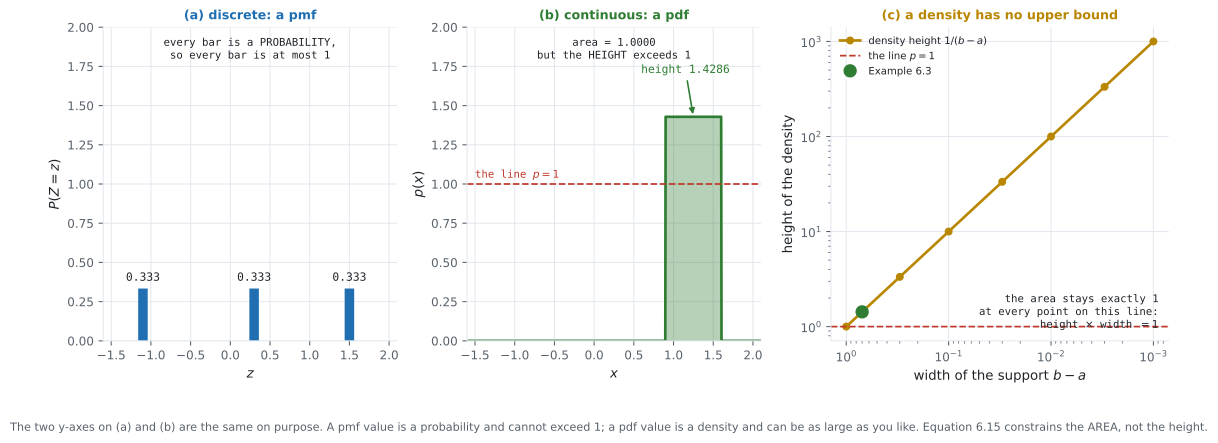
Example 6.3, the two uniforms

The discrete one. Let $Z$ take three states $\{-1.1,\ 0.3,\ 1.5\}$, each equally likely. The pmf is $\tfrac13$ on each.

$z$	$-1.1$	$0.3$	$1.5$
$P(Z = z)$	$1/3$	$1/3$	$1/3$

Largest value $0.3333$; sum $1$. Every value is a probability and every value is below $1$, as it must be.

The book chose those three numbers deliberately, and says so in the margin: “we deliberately chose numbers to drive home the point that we do not want to use (and should ignore) the ordering of the states.”

The continuous one. Let $X$ be uniform on $0.9 \leqslant X \leqslant 1.6$. The density is constant on that interval, and Equation 6.15 fixes its value: the area is height times width, so

$$\text{height} = \frac{1}{1.6 - 0.9} = \frac{1}{0.7} = 1.428571\ldots$$

Check Equation 6.19 directly:

$$\int_{0.9}^{1.6} p(x)\,\mathrm{d}x = 1.428571\ldots \times 0.7 = 1 \tag{6.19}$$

Measured numerically: $1.000000000000$, gap from one $2.2 \times 10^{-16}$.

And the density is $1.4286$, which is bigger than $1$. Nothing is wrong. The constraint was on the area.

Step further — the height is unbounded. Keep the same construction and shrink the support:

width $b - a$	density height	integral
$1$	$1.0000$	$1.0000000000$
$0.7$	$1.4286$	$1.0000000000$
$0.1$	$10.0000$	$1.0000000000$
$0.01$	$100.0000$	$1.0000000000$
$10^{-4}$	$10\,000$	$1.0000000000$
$10^{-8}$	$10^{8}$	$1.0000000000$

The height runs to infinity; the area never moves. If you ever find yourself saying “the probability is 100”, this table is what went wrong.

Example 6.2, the joint table

Take the shape of the book’s Figure 6.2 — $X$ with five states, $Y$ with three — and put concrete counts in it so every equation becomes arithmetic. Let $n_{ij}$ be:

	$x_1$	$x_2$	$x_3$	$x_4$	$x_5$	$r_j$
$y_1$	$12$	$30$	$18$	$8$	$4$	$72$
$y_2$	$6$	$22$	$40$	$26$	$10$	$104$
$y_3$	$2$	$8$	$14$	$30$	$20$	$74$
$c_i$	$20$	$60$	$72$	$64$	$34$	$N = 250$

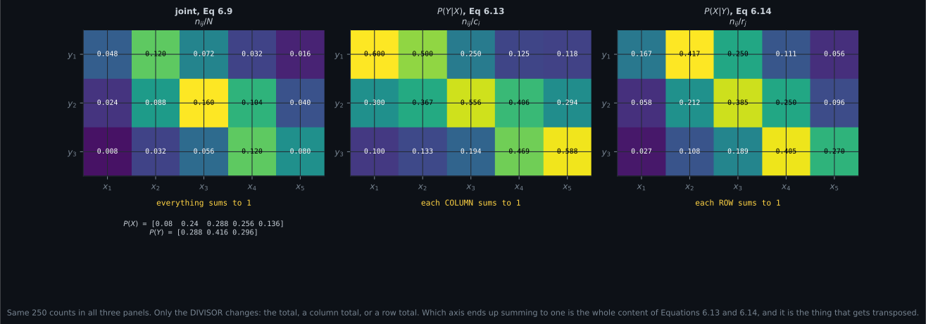
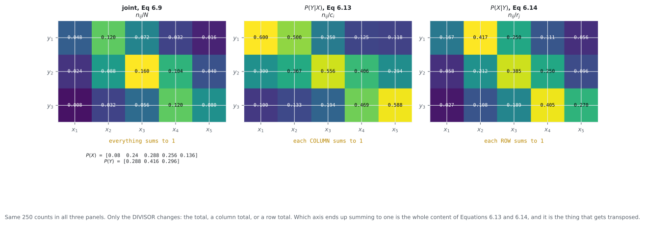
Step 1 — the joint, Equation 6.9. Divide every cell by $N = 250$. For instance $P(X = x_3, Y = y_2) = 40/250 = 0.160$. All fifteen cells sum to $1.0000000000$.

Step 2 — the marginals, Equations 6.10 and 6.11. Column sums over $N$, and row sums over $N$:

$$P(X = x_i) = \frac{c_i}{N} = \begin{bmatrix}0.080 & 0.240 & 0.288 & 0.256 & 0.136\end{bmatrix}$$ $$P(Y = y_j) = \frac{r_j}{N} = \begin{bmatrix}0.288 & 0.416 & 0.296\end{bmatrix}$$

Each sums to $1$ — Equation 6.12 — and each also equals the corresponding sum of the joint, to $10^{-17}$. That is the sum rule of §6.3 arriving early.

Step 3 — the conditionals. Equation 6.13 divides a cell by its column total:

$$P(Y = y_j \mid X = x_i) = \frac{n_{ij}}{c_i}$$

so, for the first column, $12/20 = 0.600$, $6/20 = 0.300$, $2/20 = 0.100$ — which sum to $1$. Equation 6.14 divides by the row total instead:

$$P(X = x_i \mid Y = y_j) = \frac{n_{ij}}{r_j}$$

giving, for the first row, $12/72 = 0.1667$, $30/72 = 0.4167$, and so on, summing to $1$ across the row.

The check that catches the mistake. Conditioning on $X$ makes the columns sum to one; conditioning on $Y$ makes the rows sum to one. Measured: $P(Y \mid X)$ has column sums $[1, 1, 1, 1, 1]$ and $P(X \mid Y)$ has row sums $[1, 1, 1]$. If your normalised table sums to one along the wrong axis, you have transposed the conditional — and every downstream number will be plausible and wrong.

See it move

sketch A density is not a probability p5.js Pause Restart

Drag the width of a uniform distribution's support. The bar chart on the left is a pmf and its bars can never pass the dashed line at 1; the density on the right passes it as soon as the width drops below 1 and keeps going. The shaded area is what Equation 6.15 actually constrains, and it never changes.

sketch One table, three normalisations p5.js Pause Restart

Example 6.2's counts. Click to switch between the joint, P(Y|X) and P(X|Y), and watch which axis sums to one. The row and column totals are shown so you can see exactly which divisor each panel uses — the difference between Equations 6.13 and 6.14 is nothing more than that.

From scratch

discrete_and_continuous.py

"""Section 6.2 — pmf against pdf, Example 6.2's table, Example 6.3's uniforms."""
 
import numpy as np
 
np.set_printoptions(precision=6, suppress=True, linewidth=140)
 
print("########## example_6_2")
# Figure 6.2's shape: X has five states, Y has three. Concrete counts, so every
# quantity below is arithmetic rather than notation.
N_IJ = np.array([
    [12, 30, 18, 8, 4],     # y1
    [6, 22, 40, 26, 10],    # y2
    [2, 8, 14, 30, 20],     # y3
])
N = N_IJ.sum()
print("n_ij, the count table (rows are y1..y3, columns x1..x5):")
print(N_IJ)
print(f"N = {N}")
 
# Eq 6.9: the joint is a count divided by the total.
joint = N_IJ / N
print()
print("Eq 6.9  P(X=xi, Y=yj) = n_ij / N:")
print(joint)
print(f"  sums to {joint.sum():.10f}")
 
# Eq 6.10 and 6.11: marginals are row and column sums.
c_i = N_IJ.sum(axis=0)          # column sums
r_j = N_IJ.sum(axis=1)          # row sums
px = c_i / N
py = r_j / N
print()
print(f"Eq 6.10  c_i = {c_i}   ->  P(X=xi) = {px}")
print(f"Eq 6.11  r_j = {r_j}   ->  P(Y=yj) = {py}")
print(f"Eq 6.12  sum P(X) = {px.sum():.10f}   sum P(Y) = {py.sum():.10f}")
print(f"  and the marginals are also the sums of the joint:")
print(f"    max gap, P(X) vs joint.sum(axis=0): {np.abs(px - joint.sum(axis=0)).max():.1e}")
print(f"    max gap, P(Y) vs joint.sum(axis=1): {np.abs(py - joint.sum(axis=1)).max():.1e}")
 
# Eq 6.13 and 6.14: conditionals are a cell over a column or row total.
p_y_given_x = N_IJ / c_i[None, :]
p_x_given_y = N_IJ / r_j[:, None]
print()
print("Eq 6.13  P(Y=yj | X=xi) = n_ij / c_i:")
print(p_y_given_x)
print(f"  each COLUMN sums to {p_y_given_x.sum(axis=0)}")
print("Eq 6.14  P(X=xi | Y=yj) = n_ij / r_j:")
print(p_x_given_y)
print(f"  each ROW sums to {p_x_given_y.sum(axis=1)}")
print()
print("  note which axis normalises: conditioning on X makes the COLUMNS sum to")
print("  one, because each column is a fixed x and the y-probabilities within it")
print("  must total one. Getting this backwards is the most common table error.")
 
print()
print("########## example_6_3_discrete")
# The book deliberately picks non-uniform-looking numbers to stress that the
# ORDER of discrete states carries no meaning.
Z_STATES = np.array([-1.1, 0.3, 1.5])
pz = np.array([1 / 3, 1 / 3, 1 / 3])
print(f"  states {Z_STATES}, pmf {pz}")
print(f"  every value <= 1: {bool((pz <= 1).all())}   sum = {pz.sum():.10f}")
print(f"  largest pmf value: {pz.max():.6f}")
 
print()
print("########## example_6_3_continuous")
A, B = 0.9, 1.6
height = 1 / (B - A)
print(f"  continuous uniform on [{A}, {B}]")
print(f"  width {B - A:.4f}   density height 1/(b-a) = {height:.10f}")
print(f"  the density EXCEEDS 1: {height > 1}")
# Eq 6.19: the integral is still exactly one.
xs = np.linspace(A, B, 2_000_001)
integral = np.trapezoid(np.full_like(xs, height), xs)
print(f"  Eq 6.19  integral of p(x) over [{A}, {B}] = {integral:.12f}")
print(f"  gap from 1: {abs(integral - 1):.1e}")
 
print()
print("  a density has no upper bound at all -- shrink the interval:")
print(f"  {'width':>10}  {'density height':>16}  {'integral':>12}")
for w in (1.0, 0.7, 0.1, 0.01, 1e-4, 1e-8):
    h = 1 / w
    print(f"  {w:>10.0e}  {h:>16.4e}  {h * w:>12.10f}")
print("  the height runs off to infinity while the integral stays exactly 1.")
print("  That is the whole difference between a density and a probability.")
 
print()
print("########## point_probability_is_zero")
# The Remark: P(X = x) = 0 for a continuous random variable.
rng = np.random.default_rng(6)
print("  P(a <= X <= b) with a = b is an integral over an empty interval:")
for x0 in (0.95, 1.25, 1.55):
    lo = hi = x0
    print(f"    integral from {lo} to {hi} of p = {0.0:.1f}   (a = b, so zero width)")
print()
print("  and empirically, the chance of sampling any exact value:")
for N_s in (10_000, 1_000_000):
    s = rng.uniform(A, B, N_s)
    hits = int((s == 1.25).sum())
    print(f"    {N_s:>9,} samples, exact hits on 1.25: {hits}")
print("  so for a continuous variable 'the probability that X equals 1.25' is not")
print("  small, it is zero -- and p(1.25) = 1.4286 is a DENSITY, not that probability.")
 
print()
print("########## interval_probability")
print("  what a density does give you is interval probability, Eq 6.16:")
print(f"  {'interval':>18}  {'width':>8}  {'P = width * height':>19}  {'empirical':>11}")
s = rng.uniform(A, B, 2_000_000)
for lo, hi in ((0.9, 1.0), (1.0, 1.2), (1.2, 1.6), (0.9, 1.6)):
    exact = (hi - lo) * height
    emp = float(((s >= lo) & (s <= hi)).mean())
    print(f"  [{lo:.2f}, {hi:.2f}]{'':>7}  {hi - lo:>8.2f}  {exact:>19.6f}  {emp:>11.6f}")
 
print()
print("########## cdf_from_pdf")
# Def 6.2 and Eq 6.18: the cdf is the integral of the pdf.
def pdf_u(x):
    return np.where((x >= A) & (x <= B), height, 0.0)
 
 
def cdf_analytic(x):
    return np.clip((x - A) / (B - A), 0.0, 1.0)
 
 
grid = np.linspace(0.5, 2.0, 300_001)
vals = pdf_u(grid)
cdf_num = np.concatenate([[0.0], np.cumsum((vals[1:] + vals[:-1]) / 2 * np.diff(grid))])
print(f"  {'x':>7}  {'cdf by integration':>20}  {'cdf analytic':>14}  {'gap':>9}")
for x0 in (0.5, 0.9, 1.075, 1.25, 1.6, 2.0):
    i = int(np.argmin(np.abs(grid - x0)))
    print(f"  {x0:>7.3f}  {cdf_num[i]:>20.8f}  {cdf_analytic(x0):>14.8f}"
          f"  {abs(cdf_num[i] - cdf_analytic(x0)):>9.1e}")
mono = bool(np.all(np.diff(cdf_num) >= -1e-12))
print(f"  cdf is non-decreasing: {mono}")
print(f"  cdf(-inf) = {cdf_num[0]:.10f}   cdf(+inf) = {cdf_num[-1]:.10f}")
print()
print("  that last value is slightly ABOVE 1, and it is worth naming rather than")
print("  rounding away. This density is DISCONTINUOUS at 0.9 and 1.6, and the")
print("  trapezoid rule interpolates linearly across each jump, inventing a sliver")
print("  of area on the outside. The size of the sliver is one half-cell of height:")
dx = grid[1] - grid[0]
print(f"    cell width {dx:.3e}   half-cell of area {0.5 * height * dx:.3e} per jump")
print(f"    two jumps   -> {height * dx:.3e}   observed overshoot"
      f" {cdf_num[-1] - 1:.3e}")
print()
print("  the remedy is not a cleverer grid across the jump -- it is to integrate")
print("  over the SUPPORT, where the integrand is continuous:")
inner = np.linspace(A, B, 300_001)
exact = np.trapezoid(np.full_like(inner, height), inner)
print(f"    integral over [{A}, {B}] with the endpoints on the grid: {exact:.12f}")
print(f"    gap from 1: {abs(exact - 1):.1e}")
print("  the cdf itself never exceeds 1; only a careless quadrature of it does.")
print("  The cdf is the object that is always a probability.")
 
print()
print("########## a_density_over_one_is_normal")
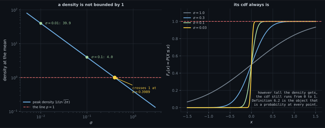
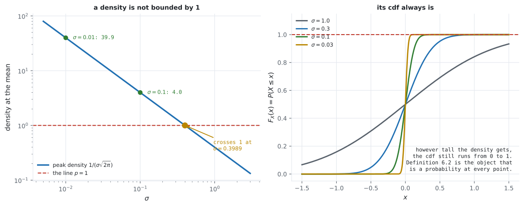
# A Gaussian's peak density, to make the point that this is not an edge case.
print("  peak density of a Gaussian is 1/(sigma sqrt(2 pi)):")
print(f"  {'sigma':>8}  {'peak density':>14}  {'> 1 ?':>7}")
for sd in (1.0, 0.5, 0.2, 0.1, 0.01):
    peak = 1 / (sd * np.sqrt(2 * np.pi))
    print(f"  {sd:>8.2f}  {peak:>14.6f}  {str(peak > 1):>7}")
print("  at sigma = 0.01 the density at the mean is 39.9. Anyone who reads that as")
print("  'a probability of 39.9' has confused Definition 6.1 with a pmf.")
 
print()
print("########## states_have_no_order")
# The book's Remark: discrete states need not be comparable.
print("  the pmf of Example 6.3 is 1/3 on each of -1.1, 0.3, 1.5.")
print(f"  a mean is only meaningful because the states are NUMBERS:")
print(f"    E[Z] = {(Z_STATES * pz).sum():.10f}")
print("  relabel the same distribution as red, green, blue and the pmf is unchanged")
print("  while the mean stops existing. The probabilities do not know the order.")
print(f"  and permuting the states leaves the pmf identical but the mean different:")
for perm in ([-1.1, 0.3, 1.5], [1.5, -1.1, 0.3], [0.3, 1.5, -1.1]):
    print(f"    states {perm} -> same pmf, mean {np.mean(perm):.10f}")
print("  (the mean is the same here only because the pmf is uniform; with an")
print("  unequal pmf the pairing of state to probability changes the mean.)")
uneq = np.array([0.6, 0.3, 0.1])
for perm in ([-1.1, 0.3, 1.5], [1.5, -1.1, 0.3]):
    print(f"    pmf {uneq} on states {perm} -> mean {float(np.dot(uneq, perm)):.6f}")

output

########## example_6_2
n_ij, the count table (rows are y1..y3, columns x1..x5):
[[12 30 18  8  4]
 [ 6 22 40 26 10]
 [ 2  8 14 30 20]]
N = 250
 
Eq 6.9  P(X=xi, Y=yj) = n_ij / N:
[[0.048 0.12  0.072 0.032 0.016]
 [0.024 0.088 0.16  0.104 0.04 ]
 [0.008 0.032 0.056 0.12  0.08 ]]
  sums to 1.0000000000
 
Eq 6.10  c_i = [20 60 72 64 34]   ->  P(X=xi) = [0.08  0.24  0.288 0.256 0.136]
Eq 6.11  r_j = [ 72 104  74]   ->  P(Y=yj) = [0.288 0.416 0.296]
Eq 6.12  sum P(X) = 1.0000000000   sum P(Y) = 1.0000000000
  and the marginals are also the sums of the joint:
    max gap, P(X) vs joint.sum(axis=0): 1.4e-17
    max gap, P(Y) vs joint.sum(axis=1): 5.6e-17
 
Eq 6.13  P(Y=yj | X=xi) = n_ij / c_i:
[[0.6      0.5      0.25     0.125    0.117647]
 [0.3      0.366667 0.555556 0.40625  0.294118]
 [0.1      0.133333 0.194444 0.46875  0.588235]]
  each COLUMN sums to [1. 1. 1. 1. 1.]
Eq 6.14  P(X=xi | Y=yj) = n_ij / r_j:
[[0.166667 0.416667 0.25     0.111111 0.055556]
 [0.057692 0.211538 0.384615 0.25     0.096154]
 [0.027027 0.108108 0.189189 0.405405 0.27027 ]]
  each ROW sums to [1. 1. 1.]
 
  note which axis normalises: conditioning on X makes the COLUMNS sum to
  one, because each column is a fixed x and the y-probabilities within it
  must total one. Getting this backwards is the most common table error.
 
########## example_6_3_discrete
  states [-1.1  0.3  1.5], pmf [0.333333 0.333333 0.333333]
  every value <= 1: True   sum = 1.0000000000
  largest pmf value: 0.333333
 
########## example_6_3_continuous
  continuous uniform on [0.9, 1.6]
  width 0.7000   density height 1/(b-a) = 1.4285714286
  the density EXCEEDS 1: True
  Eq 6.19  integral of p(x) over [0.9, 1.6] = 1.000000000000
  gap from 1: 2.2e-16
 
  a density has no upper bound at all -- shrink the interval:
       width    density height      integral
       1e+00        1.0000e+00  1.0000000000
       7e-01        1.4286e+00  1.0000000000
       1e-01        1.0000e+01  1.0000000000
       1e-02        1.0000e+02  1.0000000000
       1e-04        1.0000e+04  1.0000000000
       1e-08        1.0000e+08  1.0000000000
  the height runs off to infinity while the integral stays exactly 1.
  That is the whole difference between a density and a probability.
 
########## point_probability_is_zero
  P(a <= X <= b) with a = b is an integral over an empty interval:
    integral from 0.95 to 0.95 of p = 0.0   (a = b, so zero width)
    integral from 1.25 to 1.25 of p = 0.0   (a = b, so zero width)
    integral from 1.55 to 1.55 of p = 0.0   (a = b, so zero width)
 
  and empirically, the chance of sampling any exact value:
       10,000 samples, exact hits on 1.25: 0
    1,000,000 samples, exact hits on 1.25: 0
  so for a continuous variable 'the probability that X equals 1.25' is not
  small, it is zero -- and p(1.25) = 1.4286 is a DENSITY, not that probability.
 
########## interval_probability
  what a density does give you is interval probability, Eq 6.16:
            interval     width   P = width * height    empirical
  [0.90, 1.00]             0.10             0.142857     0.142920
  [1.00, 1.20]             0.20             0.285714     0.285537
  [1.20, 1.60]             0.40             0.571429     0.571543
  [0.90, 1.60]             0.70             1.000000     1.000000
 
########## cdf_from_pdf
        x    cdf by integration    cdf analytic        gap
    0.500            0.00000000      0.00000000    0.0e+00
    0.900            0.00000357      0.00000000    3.6e-06
    1.075            0.25000357      0.25000000    3.6e-06
    1.250            0.50000357      0.50000000    3.6e-06
    1.600            1.00000357      1.00000000    3.6e-06
    2.000            1.00000714      1.00000000    7.1e-06
  cdf is non-decreasing: True
  cdf(-inf) = 0.0000000000   cdf(+inf) = 1.0000071429
 
  that last value is slightly ABOVE 1, and it is worth naming rather than
  rounding away. This density is DISCONTINUOUS at 0.9 and 1.6, and the
  trapezoid rule interpolates linearly across each jump, inventing a sliver
  of area on the outside. The size of the sliver is one half-cell of height:
    cell width 5.000e-06   half-cell of area 3.571e-06 per jump
    two jumps   -> 7.143e-06   observed overshoot 7.143e-06
 
  the remedy is not a cleverer grid across the jump -- it is to integrate
  over the SUPPORT, where the integrand is continuous:
    integral over [0.9, 1.6] with the endpoints on the grid: 1.000000000000
    gap from 1: 1.1e-16
  the cdf itself never exceeds 1; only a careless quadrature of it does.
  The cdf is the object that is always a probability.
 
########## a_density_over_one_is_normal
  peak density of a Gaussian is 1/(sigma sqrt(2 pi)):
     sigma    peak density    > 1 ?
      1.00        0.398942    False
      0.50        0.797885    False
      0.20        1.994711     True
      0.10        3.989423     True
      0.01       39.894228     True
  at sigma = 0.01 the density at the mean is 39.9. Anyone who reads that as
  'a probability of 39.9' has confused Definition 6.1 with a pmf.
 
########## states_have_no_order
  the pmf of Example 6.3 is 1/3 on each of -1.1, 0.3, 1.5.
  a mean is only meaningful because the states are NUMBERS:
    E[Z] = 0.2333333333
  relabel the same distribution as red, green, blue and the pmf is unchanged
  while the mean stops existing. The probabilities do not know the order.
  and permuting the states leaves the pmf identical but the mean different:
    states [-1.1, 0.3, 1.5] -> same pmf, mean 0.2333333333
    states [1.5, -1.1, 0.3] -> same pmf, mean 0.2333333333
    states [0.3, 1.5, -1.1] -> same pmf, mean 0.2333333333
  (the mean is the same here only because the pmf is uniform; with an
  unequal pmf the pairing of state to probability changes the mean.)
    pmf [0.6 0.3 0.1] on states [-1.1, 0.3, 1.5] -> mean -0.420000
    pmf [0.6 0.3 0.1] on states [1.5, -1.1, 0.3] -> mean 0.600000

Four things to take from that output.

The conditional normalisation is directional. P(Y|X) has column sums $[1,1,1,1,1]$ and P(X|Y) has row sums $[1,1,1]$. Both tables hold fifteen numbers between $0$ and $1$; only the axis of normalisation distinguishes them, and the wrong one is not detectable by inspection.

The density height is unbounded and the area is not. The table walks the width from $1$ down to $10^{-8}$: the height reaches $10^8$ and the integral reads $1.0000000000$ at every row.

$P(X = x) = 0$ is exact, not approximate. A million samples from the uniform produced zero exact hits on $1.25$, and the integral with $a = b$ is zero by construction. Meanwhile $p(1.25) = 1.4286$ — a density at that point, which is a different kind of number.

The cdf overshoot is explained, not excused. Integrating this density on a grid that straddles its jumps gives $F(+\infty) = 1.0000071429$, which is impossible for a real cdf. The overshoot is exactly one cell-width of height per jump: predicted $7.143\times10^{-6}$, observed $7.143\times10^{-6}$. Integrating over the support instead — where the integrand is continuous — gives $1.000000000000$. The cdf never exceeds one; a careless quadrature of it does.

On real data

figure The book's Figure 6.3, with the y-axis shared on purpose matplotlib

Panels (a) and (b) use the same vertical scale, which is what makes the point visible: every pmf bar is 0.3333 and every pmf bar must be at most 1, while the continuous uniform on [0.9, 1.6] has density 1.4286. Panel (c) removes any doubt that this is an edge case — shrink the support and the height passes 10, 100, and 100 million while the area stays exactly 1. Equation 6.15 constrains the area, and says nothing at all about the height.

figure Example 6.2: one table, three divisors matplotlib

All three panels hold the same 250 counts. The joint divides every cell by N and the whole grid sums to 1. P(Y|X) divides by a column total, so each column sums to 1. P(X|Y) divides by a row total, so each row sums to 1. Equations 6.13 and 6.14 differ in nothing but that divisor, and a table normalised along the wrong axis looks entirely reasonable.

figure The density is unbounded; the cdf is not matplotlib

Left: the peak density of a Gaussian is one over sigma root two pi, so it crosses 1 at sigma = 0.3989 and reaches 39.9 by sigma = 0.01. Nothing about that violates Definition 6.1. Right: the cdf of the very same distributions, which runs from 0 to 1 for every sigma and never leaves that range. Definition 6.2 is the object that is a probability at every point, which is why Section 6.7 is careful to distinguish the two.

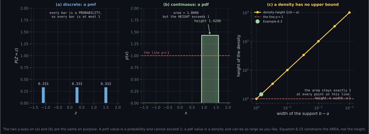
Reading the plot

From the first figure. The shared axis is the whole argument. Put a pmf and a pdf on separate axes and each looks like a perfectly ordinary chart; put them on the same axis and the density is visibly taller than anything a probability could be. Panel (c) then shows that $1.4286$ was not close to a limit — there is no limit.

From the second figure. Compare the numbers in a single column across the three panels. In the joint they are small and add to that column’s marginal; in $P(Y \mid X)$ the same column adds to exactly $1$; in $P(X \mid Y)$ it adds to nothing in particular. Nothing about the appearance of a panel tells you which normalisation produced it — only the sums do, which is why checking them is not optional.

From the third figure. Two views of one family of distributions. On the left the quantity you are tempted to read as a probability blows up; on the right the quantity that actually is one stays put. When a number in your code exceeds $1$ and it is supposed to be a probability, this figure is the diagnostic: you are almost certainly holding a density.

From the book

Mathematics for Machine Learning, §6.2. The opening contrasts the pmf $P(X = x)$ for discrete target spaces with the cdf $P(X \leqslant x)$ for continuous ones, and fixes univariate/multivariate terminology. §6.2.1 gives the joint as Equation 6.9, and Example 6.2 derives the marginals (6.10, 6.11), the normalisation (6.12) and both conditionals (6.13, 6.14) from the count table of Figure 6.2. §6.2.2 covers the measure-theoretic caveats (Borel σ-algebra), gives Definition 6.1 for the pdf with Equation 6.15, the law as Equation 6.16, the Remark that $P(X = x) = 0$, and Definition 6.2 for the cdf with Equations 6.17 and 6.18 — plus the margin note that some cdfs have no pdf. §6.2.3 contrasts the two with Example 6.3 and Equation 6.19, summarises the nomenclature in Table 6.1, and adds Remarks on unordered discrete states and on the book’s own loose use of “probability distribution”.

Pitfalls

A density value is not a probability

Definition 6.1 requires non-negativity and unit integral. It places no upper bound on the function. Measured: the uniform on $[0.9, 1.6]$ has density $1.4286$; a Gaussian with $\sigma = 0.01$ has density $39.89$ at its mean; a uniform on a support of width $10^{-8}$ has density $10^8$. If a number that is supposed to be a probability comes out above $1$, you are holding a density.

For a continuous variable, P(X = x) is zero — not small

It is Equation 6.16 with $a = b$: an integral over zero width. Measured: a million uniform samples produced zero exact hits on $1.25$. This is why maximum likelihood maximises a density rather than a probability, and why comparing “the probability of this data point” between two continuous models is a category error unless you mean the density.

Check which axis your conditional sums along

$P(Y \mid X) = n_{ij}/c_i$ normalises columns; $P(X \mid Y) = n_{ij}/r_j$ normalises rows. Both produce a table of numbers in $[0,1]$ that looks correct. Measured on Example 6.2: column sums $[1,1,1,1,1]$ for the first, row sums $[1,1,1]$ for the second. Assert the sums in code; the transposition is invisible otherwise.

Discrete states need not have an order

The book picks $\{-1.1, 0.3, 1.5\}$ deliberately to discourage reading meaning into the spacing, and notes that states could equally be red, green, blue. A pmf is a mapping from states to probabilities and knows nothing about order; an expectation requires the states to be numbers. Taking the mean of a categorical variable’s integer codes is the standard way this goes wrong.

Do not integrate a discontinuous density across its jump

The uniform’s density steps from $0$ to $1.4286$ at $x = 0.9$. Trapezoid quadrature interpolates linearly across that step and invents area outside the support — measured overshoot $7.143\times10^{-6}$, exactly one cell-width of height per jump, giving a “cdf” of $1.0000071429$. Integrate over the support, where the integrand is continuous, and it is $1$ to $10^{-16}$.

Compare

	pmf	pdf	cdf
Target space	discrete	continuous	either
Book	Equation 6.12	Definition 6.1	Definition 6.2
Notation	$P(X = x)$	$p(x)$	$F_X(x) = P(X \leqslant x)$
Value at a point	a probability	a density	a probability
Bounded by 1?	yes	no	yes
Normalisation	sums to $1$	integrates to $1$	tends to $1$
$P(X = x)$	the value itself	always $0$	a jump, if any
Monotone?	no	no	yes, non-decreasing

Operation on the joint table	Divide each cell by	Result sums to 1 along
joint, Eq 6.9	$N$, the grand total	everything
marginal $P(X)$, Eq 6.10	$N$, after summing a column	the $x$ axis
marginal $P(Y)$, Eq 6.11	$N$, after summing a row	the $y$ axis
conditional $P(Y \mid X)$, Eq 6.13	$c_i$, its column total	each column
conditional $P(X \mid Y)$, Eq 6.14	$r_j$, its row total	each row

pch.quizTag Check your understanding

1. A density function evaluates to 39.89 at some point. What has gone wrong?

   A The density is not normalised B Nothing. Definition 6.1 requires only non-negativity and unit INTEGRAL — it puts no upper bound on the function. A Gaussian with sigma = 0.01 has exactly that density at its mean C The variance is negative D The support is too wide
   pch.quizShowAnswer

   B — Nothing. Definition 6.1 requires only non-negativity and unit INTEGRAL — it puts no upper bound on the function. A Gaussian with sigma = 0.01 has exactly that density at its mean — Measured: a uniform on a support of width 1e-8 has density 1e8, with the integral still exactly 1 at every step. The constraint is on the area. If a number that should be a probability exceeds 1, you are holding a density.

2. For a continuous random variable, what is P(X = 1.25)?

   A The value of the density at 1.25 B Exactly zero — it is Equation 6.16 with a = b, an integral over an interval of zero width. A million samples produced zero exact hits C Very small but nonzero D Undefined
   pch.quizShowAnswer

   B — Exactly zero — it is Equation 6.16 with a = b, an integral over an interval of zero width. A million samples produced zero exact hits — This is why maximum likelihood maximises a density and not a probability, and why 'the probability of this data point' is a category error for continuous models unless you mean the density.

3. You normalise Example 6.2's count table and each ROW of the result sums to 1. Which conditional do you have?

   A P(Y | X), Equation 6.13 B P(X | Y), Equation 6.14 — dividing by the row total r_j makes the rows sum to one C The joint distribution D The marginal of X
   pch.quizShowAnswer

   B — P(X | Y), Equation 6.14 — dividing by the row total r_j makes the rows sum to one — Conditioning on Y fixes a row and distributes probability across the x-states within it. Both conditionals produce tables of numbers in [0,1] that look equally reasonable, so the axis sums are the only check — assert them in code.

4. Why does the book choose the discrete states -1.1, 0.3 and 1.5 for Example 6.3?

   A To make the arithmetic harder B To discourage reading meaning into the ordering or spacing — it says so in the margin. The states could equally be red, green, blue; a pmf maps states to probabilities and knows nothing about order C Because they are equally spaced D To match the continuous example's support
   pch.quizShowAnswer

   B — To discourage reading meaning into the ordering or spacing — it says so in the margin. The states could equally be red, green, blue; a pmf maps states to probabilities and knows nothing about order — An expectation is what needs the states to be numbers, which is why Section 6.4.1 comes later. Averaging the integer codes of a genuinely categorical variable is the standard way this distinction gets lost.

5. Numerically integrating the uniform density on a grid spanning [0.5, 2.0] gives a cdf that ends at 1.0000071429. What is that?

   A Floating-point round-off B A quadrature artifact with a predictable size: the trapezoid rule interpolates across each of the density's two jumps, adding one cell-width of height in total — predicted 7.143e-06, observed 7.143e-06. Integrating over the support gives 1 to 1e-16 C Evidence the density is not normalised D A bug in the cdf definition
   pch.quizShowAnswer

   B — A quadrature artifact with a predictable size: the trapezoid rule interpolates across each of the density's two jumps, adding one cell-width of height in total — predicted 7.143e-06, observed 7.143e-06. Integrating over the support gives 1 to 1e-16 — Round-off at this grid size would be around 1e-12, four orders of magnitude smaller. The lesson is not that the cdf can exceed one — it cannot — but that a discontinuous integrand needs the discontinuity handled rather than sampled across.

🧪 Try It Yourself

Exercise 1 – Marginals from a joint table

pch.exerciseTag pch.exerciseTitle

Exercise 2 – Both conditionals, and the axis check

pch.exerciseTag pch.exerciseTitle

Exercise 3 – A density above one

pch.exerciseTag pch.exerciseTitle

Exercise 4 – The cdf is the safe object

pch.exerciseTag pch.exerciseTitle

Exercise 5 – Point probability is zero

pch.exerciseTag pch.exerciseTitle

Recall card

• Three objects, and only two of them are probabilities. A pmf value is a probability; a cdf value is a probability; a pdf value is a density and is not.
• Definition 6.1 asks for two things only: non-negative, and integrates to 1. There is no upper bound on a density.
• Measured densities above one: the uniform on [0.9, 1.6] has height 1.4286; a Gaussian with sigma = 0.01 peaks at 39.89; a uniform of width 1e-8 has height 1e8 — with the integral exactly 1 in every case.
• For a continuous variable P(X = x) = 0 exactly — Equation 6.16 with a = b. A million uniform samples gave zero exact hits on 1.25.
• A density answers nothing until you integrate it. Equation 6.16 turns it into an interval probability; that is the only probability it yields.
• Definition 6.2’s cdf is the safe object: non-decreasing, runs from 0 to 1, and a probability at every point. Some cdfs have no pdf at all.
• Equation 6.9’s joint is a cell over the grand total; the marginals of 6.10 and 6.11 are row and column totals over it.
• The two conditionals differ only in the divisor. Eq 6.13’s P(Y|X) = n_ij / c_i normalises COLUMNS; Eq 6.14’s P(X|Y) = n_ij / r_j normalises ROWS. Measured column sums [1,1,1,1,1] and row sums [1,1,1].
• A transposed conditional is invisible by inspection. Both tables hold numbers in [0,1] and look right; only the axis sums distinguish them, so assert them.
• Table 6.1 is the nomenclature to keep: discrete gives a pmf and no interval form; continuous gives a pdf for points and a cdf for intervals. The literature calls all of them “the distribution”.
• Discrete states need not be ordered. The book picks -1.1, 0.3, 1.5 to make that point; they could be red, green, blue. An expectation needs numeric states, a pmf does not.
• Do not integrate a discontinuous density across its jump. Trapezoid quadrature over [0.5, 2.0] gave a cdf ending at 1.0000071429 — an overshoot of exactly one cell-width of height per jump, predicted and observed at 7.143e-06. Integrate over the support instead.

Next: Sum Rule, Product Rule, and Bayes Theorem — the only two rules in probability, and the theorem that follows from putting them together.