Notation and Symbols

Most of the difficulty in reading a mathematics textbook for the first time is not the mathematics. It is that the author fixed a notation in the front matter, assumed you memorised it, and then wrote four hundred pages in it. Miss one convention and a page that would have been easy becomes unreadable.

This page is that front matter, expanded. It mirrors the Table of Symbols in Mathematics for Machine Learning (pages 6 and 7), adds the chapter where each symbol first does real work, and flags the half-dozen places where the same mark means two different things.

Bookmark it. You will come back.

What you’ll learn

• The typeface convention that tells you a scalar from a vector from a matrix, at a glance.
• Why $\mathbf{x}^\top\mathbf{y}$ and $\langle\mathbf{x},\mathbf{y}\rangle$ are written differently even when they are equal.
• The difference between $B$, $\boldsymbol{B}$ and $\mathcal{B}$, which the book uses on the same page.
• Which symbols are overloaded, and how to tell from context which meaning is in play.
• Where each symbol first appears, so you can look up the derivation rather than the definition.

The one convention that matters most

Everything else is lookup. This one is worth memorising:

you see	it is a	example
lowercase italic	scalar — a single number	$a$, $b$, $c$, $\alpha$, $\beta$, $\gamma$, $\lambda$
lowercase bold	vector — a column of numbers	$\mathbf{x}$, $\mathbf{y}$, $\mathbf{z}$, $\mathbf{b}_1$
uppercase bold	matrix — a grid of numbers	$\mathbf{A}$, $\mathbf{B}$, $\mathbf{C}$
uppercase italic	a count, or a random variable	$D$, $N$, $X$, $Y$
calligraphic	a set	$\mathcal{A}$, $\mathcal{B}$, $\mathcal{C}$

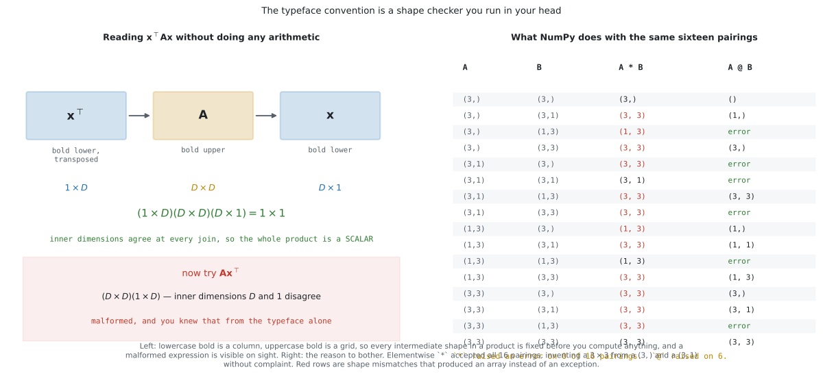
So $\mathbf{x}^\top\mathbf{A}\mathbf{x}$ reads immediately as row-vector times matrix times column-vector, which must come out a scalar. Reading shapes off the typeface is how you catch an error in a derivation without doing any arithmetic, and it is the single most useful habit this page can give you.

The one that catches everyone

$B$, $\boldsymbol{B}$ and $\mathcal{B}$ are three different objects and the book uses all three:

• $B = (\mathbf{b}_1, \mathbf{b}_2, \mathbf{b}_3)$ — an ordered tuple of vectors. Order matters.
• $\boldsymbol{B} = [\mathbf{b}_1, \mathbf{b}_2, \mathbf{b}_3]$ — a matrix whose columns are those vectors.
• $\mathcal{B} = \{\mathbf{b}_1, \mathbf{b}_2, \mathbf{b}_3\}$ — an unordered set of vectors.

A basis is a tuple when you care about coordinate order, a matrix when you want to multiply by it, and a set when you only care about membership. Same three vectors, three jobs.

Vectors and matrices

symbol	meaning	first used
$\mathbf{x}^\top$, $\mathbf{A}^\top$	transpose: rows become columns	2.2 Matrices
$\mathbf{A}^{-1}$	inverse of a matrix	2.2 Matrices
$\langle\mathbf{x},\mathbf{y}\rangle$	inner product of $\mathbf{x}$ and $\mathbf{y}$	3.2 Inner Products
$\mathbf{x}^\top\mathbf{y}$	dot product of $\mathbf{x}$ and $\mathbf{y}$	2.2 Matrices
$\mathbf{I}_m$	identity matrix, size $m\times m$	2.2 Matrices
$\mathbf{0}_{m,n}$	matrix of zeros, size $m\times n$	2.2 Matrices
$\mathbf{1}_{m,n}$	matrix of ones, size $m\times n$	2.2 Matrices
$\mathbf{e}_i$	standard basis vector: $1$ in component $i$, zero elsewhere	2.6 Basis and Rank
$\dim$	dimension of a vector space	2.6 Basis and Rank
$\operatorname{rk}(\mathbf{A})$	rank of $\mathbf{A}$	2.6 Basis and Rank
$\operatorname{Im}(\Phi)$	image of a linear mapping $\Phi$	2.7 Linear Mappings
$\ker(\Phi)$	kernel, or null space, of $\Phi$	2.7 Linear Mappings
$\operatorname{span}[\mathbf{b}_1]$	span, the set of all multiples and combinations	2.4 Vector Spaces
$\operatorname{tr}(\mathbf{A})$	trace: the sum of the diagonal	4.1 Determinant and Trace
$\det(\mathbf{A})$	determinant	4.1 Determinant and Trace
$E_\lambda$	eigenspace for eigenvalue $\lambda$	4.2 Eigenvalues and Eigenvectors

Two notes worth having in advance.

Why both $\langle\cdot,\cdot\rangle$ and $\mathbf{x}^\top\mathbf{y}$? The dot product is one inner product — the standard one. $\langle\cdot,\cdot\rangle$ is the general notion, and Chapter 3 builds real geometry from any of them, including inner products on spaces of functions where there are no components to multiply pairwise. When the book writes angle brackets it is telling you the argument does not depend on the standard choice.

Why $\mathbf{e}_i$ deserves its own symbol. Once you have it, the columns of a matrix are just $\mathbf{A}\mathbf{e}_i$, and half of Chapter 2 becomes one sentence: a matrix is where the basis vectors go.

Number systems

symbol	meaning
$\mathbb{N}$	natural numbers
$\mathbb{Z}$	integers
$\mathbb{R}$	real numbers
$\mathbb{C}$	complex numbers
$\mathbb{R}^n$	the $n$-dimensional vector space of real column vectors
$\mathbb{R}^{m\times n}$	all real matrices with $m$ rows and $n$ columns

$\mathbb{R}^n$ is the single most common symbol in the book. Read it as “a list of $n$ real numbers, which we are treating as a point and as an arrow at the same time”.

$\mathbb{C}$ appears rarely, and always for one reason: a real matrix can have complex eigenvalues. A rotation is the standard example, and Complex Numbers in One Page covers exactly as much as you need.

Logic, sets and definitions

symbol	meaning
$\forall x$	for all $x$
$\exists x$	there exists an $x$
$a := b$	$a$ is defined to be $b$
$a =: b$	$b$ is defined to be $a$
$a \propto b$	$a$ is proportional to $b$: $a = \text{const}\cdot b$
$g \circ f$	function composition: ”$g$ after $f$”
$\Longleftrightarrow$	if and only if
$\Longrightarrow$	implies
$\mathcal{A}$, $\mathcal{C}$	sets
$a \in \mathcal{A}$	$a$ is an element of $\mathcal{A}$
$\emptyset$	the empty set

Colon-equals means defined as; plain equals means asserted equal

$a := b$ introduces a name. $a = b$ claims a fact. In a derivation, an $=$ is something you may have to prove and a $:=$ never is, so the distinction tells you which lines carry the argument. Very few textbooks bother; this one does, and it is a real convenience.

$\propto$ does the same job for probability: writing $p(\theta \mid x) \propto p(x \mid \theta)p(\theta)$ says “up to a constant that does not depend on $\theta$”, which is exactly the constant nobody wants to compute. It appears constantly from §6.3 onward.

Counting and indexing

symbol	meaning
$D$	number of dimensions, indexed $d = 1,\dots,D$
$N$	number of data points, indexed $n = 1,\dots,N$

This pairing is fixed throughout the book, and it is worth internalising because it disambiguates almost every summation you will meet: $\sum_{n=1}^{N}$ runs over examples, and $\sum_{d=1}^{D}$ runs over features. When you see a double sum, the outer index tells you what the quantity is per.

Calculus

symbol	meaning	first used
$\frac{\partial f}{\partial x}$	partial derivative of $f$ with respect to $x$	5.2 Partial Differentiation
$\frac{\mathrm{d}f}{\mathrm{d}x}$	total derivative of $f$ with respect to $x$	5.1 Differentiation
$\nabla$	gradient	5.2 Partial Differentiation
$\boldsymbol{\theta}$	parameter vector — the thing being learned	8.1 Data, Models, Learning
$\mathfrak{L}$	Lagrangian	7.2 Lagrange Multipliers
$\mathcal{L}$	negative log-likelihood	8.3 Parameter Estimation

Two overloads to watch

$\lambda$ means two things. In Chapter 4 it is an eigenvalue. In Chapter 7 it is a Lagrange multiplier, and in Chapter 9 a regularisation strength. Context always makes it clear, but if a line stops making sense, check which $\lambda$ you are reading.

$\mathfrak{L}$ and $\mathcal{L}$ are different letters. Fraktur $\mathfrak{L}$ is the Lagrangian of a constrained optimisation problem; calligraphic $\mathcal{L}$ is a negative log-likelihood. They appear two chapters apart and mean unrelated things.

$|\cdot|$ means absolute value or determinant, depending on whether the argument is a number or a matrix. The book says so explicitly in its table. $\lVert\cdot\rVert$ is a norm — Euclidean unless a subscript says otherwise.

Probability and statistics

symbol	meaning	first used
$X \sim p$	the random variable $X$ is distributed according to $p$	6.2 Discrete and Continuous
$\mathbb{E}_X[\mathbf{x}]$	expectation of $\mathbf{x}$ with respect to $X$	6.4 Summary Statistics
$\mathbb{V}_X[\mathbf{x}]$	variance of $\mathbf{x}$ with respect to $X$	6.4 Summary Statistics
$\operatorname{Cov}_{X,Y}[\mathbf{x},\mathbf{y}]$	covariance between $\mathbf{x}$ and $\mathbf{y}$	6.4 Summary Statistics
$X \perp\!\!\!\perp Y \mid Z$	$X$ is conditionally independent of $Y$ given $Z$	6.4, 8.5 Graphical Models
$\binom{n}{k}$	binomial coefficient, ”$n$ choose $k$”	6.2 Discrete and Continuous
$\mathcal{N}(\boldsymbol{\mu},\boldsymbol{\Sigma})$	Gaussian with mean $\boldsymbol{\mu}$, covariance $\boldsymbol{\Sigma}$	6.5 Gaussian Distribution
$\mathrm{Ber}(\mu)$	Bernoulli distribution with parameter $\mu$	6.2 Discrete and Continuous
$\mathrm{Bin}(N,\mu)$	Binomial with parameters $N$ and $\mu$	6.2 Discrete and Continuous
$\mathrm{Beta}(\alpha,\beta)$	Beta distribution with parameters $\alpha$, $\beta$	6.6 Conjugacy

The subscript on $\mathbb{E}_X$ is not decoration. When a quantity depends on two random variables, $\mathbb{E}_X[f(X, Y)]$ averages over $X$ and leaves a function of $Y$; dropping the subscript makes the expression ambiguous. Every derivation in Chapters 8 to 11 leans on this.

Abbreviations

acronym	meaning
i.i.d.	independent, identically distributed
MLE	maximum likelihood estimation, or estimator
MAP	maximum a posteriori
ONB	orthonormal basis
REF	row-echelon form
SPD	symmetric, positive definite
PCA	principal component analysis
PPCA	probabilistic principal component analysis
GMM	Gaussian mixture model
SVM	support vector machine
e.g.	exempli gratia — for example
i.e.	id est — that is

SPD is worth flagging early. “Symmetric positive definite” is a mouthful that turns up on almost every page from Chapter 3 onward, because it is precisely the condition for a matrix to define an inner product (§3.2), to have a Cholesky factorisation (§4.3), to be a valid covariance matrix (§6.4), and for a quadratic objective to be convex (§7.3). One property, five uses.

How the book cross-references itself

you see	it means
Definition 2.4	a definition, numbered within its chapter
Theorem 4.15	a claim with a proof
Example 3.5	a worked instance
(3.41)	equation 41 of Chapter 3
Remark	a side comment, often the most useful paragraph on the page

Every page in this module ends with a From the book box citing these numbers, so you can read the page and the PDF side by side without hunting.

See it move

The convention is only worth memorising if you can run it. Drag the knobs to build a product out of two operands, and read off whether the typefaces you chose can legally be multiplied at all — before any numbers exist.

sketch Read the shape off the typeface p5.js Pause Restart

Pick a typeface for each operand and whether it is transposed. The sketch works out the shape of each operand from its typeface alone, checks the inner dimensions, and tells you whether the product is legal and what it returns. No arithmetic is involved anywhere.

On real data

figure The typeface convention is a shape checker you run in your head matplotlib

Every intermediate shape in the product is fixed by the typeface before any arithmetic happens, so a malformed expression is visible on sight. NumPy will not do this for you: elementwise multiplication accepted all sixteen pairings, including turning a (3,) and a (3,1) into a (3,3).

figure One basis, three objects matplotlib

A basis is a tuple when coordinates need a fixed order, a matrix when you want to multiply by it, and a set when only membership matters. Asking for the second element of the set is not a typo, it is a question the object cannot answer.

figure Six marks that mean more than one thing matplotlib

In every case it is the type of the argument that settles the meaning, never the mark itself. Single bars around a scalar are absolute value, around a square matrix a determinant, around a set a cardinality.

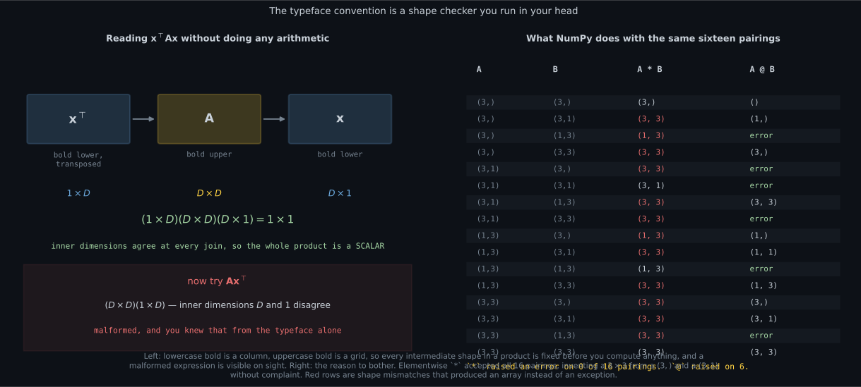
Reading the plot

The first figure is the convention doing work. Read the left panel left to right and notice that no numbers appear anywhere. $\mathbf{x}^\top$ is lowercase bold and transposed, so it is $1 \times D$; $\mathbf{A}$ is uppercase bold, so it is $D \times D$; $\mathbf{x}$ is $D \times 1$. Each join has matching inner dimensions, the outer dimensions are $1$ and $1$, and therefore $\mathbf{x}^\top\mathbf{A}\mathbf{x}$ is a scalar. The red box below shows the same reading applied to $\mathbf{A}\mathbf{x}^\top$: $(D \times D)(1 \times D)$, inner dimensions $D$ and $1$, malformed. You did not need to know a single entry of either object to say that.

The right panel is the reason this is a habit worth having rather than a nicety. It runs all sixteen pairings of the shapes (3,), (3,1), (1,3) and (3,3) through both operators. @ refuses six of them, which is helpful. * refuses none. All sixteen returned an array. Twelve of those sixteen were between shapes that are not equal, and the worst case is the pairing highlighted in the caption: a (3,) times a (3,1) returns a (3,3) — an outer product where almost anyone writing that line meant an elementwise one. There is no exception, no warning, and the downstream code will happily consume a matrix where a vector belonged. The typeface convention is the check that catches this, because it fixes the intended shape at the point where you write the mathematics.

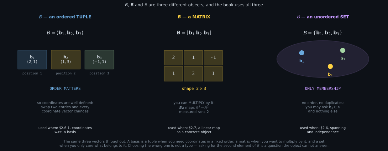
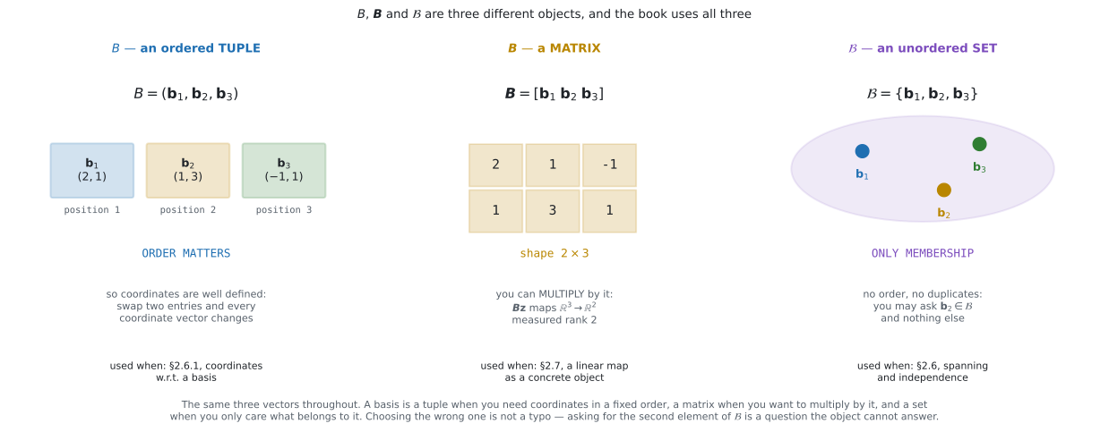
The second figure is the $B$ / $\boldsymbol{B}$ / $\mathcal{B}$ distinction made concrete. The same three vectors appear in all three panels. As a tuple they have positions, which is what makes “the coordinates of $\mathbf{v}$ with respect to $B$” a well-defined phrase — permute the tuple and every coordinate vector changes. As a matrix they have a shape, here $2 \times 3$ and measured rank $2$, and you can multiply by it. As a set they have only membership: three elements, no first element, no order. The reason the book keeps all three rather than picking one is that each throws away exactly what the other two need to keep, and each of §2.6, §2.6.1 and §2.7 needs a different one.

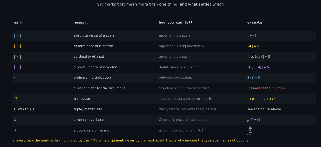
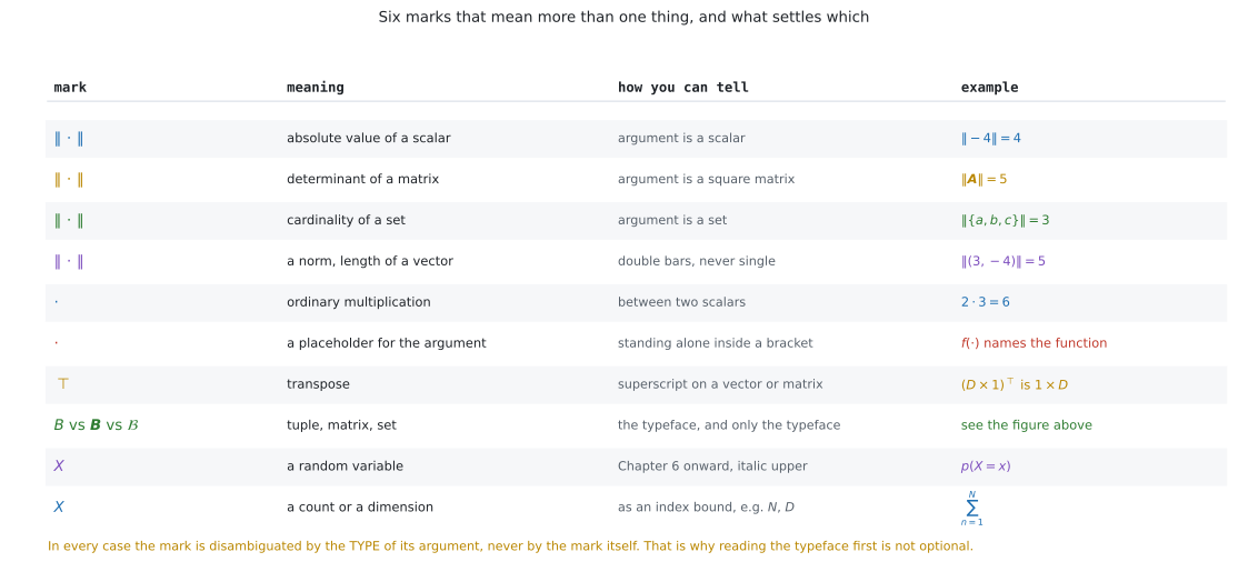
The third figure is the lookup table for ambiguity, and it has one structural lesson. Scan the third column. Every disambiguating cue is a fact about the argument, not about the mark: single bars mean absolute value around a scalar, a determinant around a square matrix, a cardinality around a set. The centred dot is multiplication between two things and a placeholder when it stands alone. Italic uppercase is a random variable in Chapter 6 and a count when it bounds a sum. So the marks are not really ambiguous once you have read the typefaces — which is the argument for doing that first, and the reason this page puts the typeface table above everything else.

From the book

This page mirrors the Table of Symbols (pages 6 and 7 of the December 2019 draft) and the Table of Abbreviations and Acronyms (page 7) of Mathematics for Machine Learning by Deisenroth, Faisal and Ong. The typeface convention for scalars, vectors and matrices, the three-way distinction between $B$, $\boldsymbol{B}$ and $\mathcal{B}$, the $D$/$N$ indexing convention, and the explicit note that $|\cdot|$ is “absolute value or determinant depending on context” are all taken directly from those tables. The chapter attributions in the right-hand columns are this module’s addition.

pch.quizTag Can you read the notation?

1. You read an expression and see a bold lowercase letter multiplied by a bold uppercase letter. What is the result?

   A A scalar, always B It depends on the order and the shapes, but bold lowercase is a vector and bold uppercase is a matrix C A matrix, always D The notation is invalid
   pch.quizShowAnswer

   B — It depends on the order and the shapes, but bold lowercase is a vector and bold uppercase is a matrix — Bold lowercase is a vector, bold uppercase is a matrix. Whether the product is a vector or a scalar depends on the shapes and on which side the vector sits, and reading that off the typeface is exactly the habit the convention exists to give you.

2. In a derivation you see a line beginning with a colon-equals rather than a plain equals sign. What does that tell you?

   A The line is an approximation B The line introduces a definition, so there is nothing to prove there C The line is a claim that needs a proof D The two sides are proportional rather than equal
   pch.quizShowAnswer

   B — The line introduces a definition, so there is nothing to prove there — Colon-equals introduces a name. Plain equals asserts a fact you may have to justify. Scanning a derivation for plain equals signs shows you where the actual argument lives.

3. The symbol lambda appears in Chapter 4 and again in Chapter 7. What has changed?

   A Nothing — it means the same thing throughout the book B It is an eigenvalue in Chapter 4 and a Lagrange multiplier in Chapter 7 C It is a Lagrange multiplier in Chapter 4 and an eigenvalue in Chapter 7 D Chapter 7 uses a different letter
   pch.quizShowAnswer

   B — It is an eigenvalue in Chapter 4 and a Lagrange multiplier in Chapter 7 — The book's own symbol table lists lambda as eigenvalue or Lagrange multiplier. Chapter 10 then uses both at once when it derives PCA by maximising variance under a constraint, so knowing the overload exists matters.

4. What does the subscript in an expectation such as E-sub-X tell you?

   A Which variable is being averaged over, leaving the others as free variables B The number of samples used C That the expectation is over the training set only D Nothing — it is conventional decoration
   pch.quizShowAnswer

   A — Which variable is being averaged over, leaving the others as free variables — It names the variable being integrated out. With two random variables in play, the expectation over one leaves a function of the other, and without the subscript the expression is ambiguous.

🧪 Try It Yourself

Exercise 1 – Read the shape, then check it

pch.exerciseTag pch.exerciseTitle

Exercise 2 – One mark, four meanings

pch.exerciseTag pch.exerciseTitle

Exercise 3 – Tuple, matrix, set

pch.exerciseTag pch.exerciseTitle

Exercise 4 – The trap the typeface exists to prevent

pch.exerciseTag pch.exerciseTitle

Exercise 5 – The N-by-D convention, and why it is a convention

pch.exerciseTag pch.exerciseTitle

Recall card

• Typeface rule — lowercase italic is a scalar, lowercase bold a vector, uppercase bold a matrix, calligraphic a set, uppercase italic a count or a random variable.
• := introduces a definition, = asserts a fact you may have to prove — which is how you find where a derivation’s real argument lives.
• The three B’s are three different objects: a tuple of vectors, the matrix with those columns, and the unordered set.
• The absolute-value bars mean determinant when the argument is a matrix — the double bars are the norm, Euclidean unless subscripted.
• Lambda is an eigenvalue in Chapter 4 and a Lagrange multiplier in Chapter 7 — and PCA uses both meanings on one page.
• N indexes data points and D indexes dimensions — so the outer index of a double sum tells you what the quantity is measured per.
• SPD means symmetric positive definite — the condition for an inner product, a Cholesky factorisation, a valid covariance and a convex quadratic.

Next: the notation you will use most often, and the manipulations that go with it — Sums, Products, and Set Notation.