The Latent Variable Perspective

Everything so far has worked without a story. §11.4 supplies one, and is explicit that it is not decoration:

The advantages of the probabilistic perspective are that (i) it will justify some ad hoc decisions we made in the previous sections, (ii) it allows for a concrete interpretation of the responsibilities as posterior probabilities, and (iii) the iterative algorithm for updating the model parameters can be derived in a principled manner.

All three are checkable, and this page checks them.

What you’ll learn

Equations 11.58–11.62: the one-hot latent $\mathbf{z}$ , the prior $p(\mathbf{z}) = \boldsymbol\pi$ , and the joint.
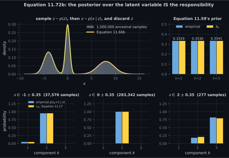
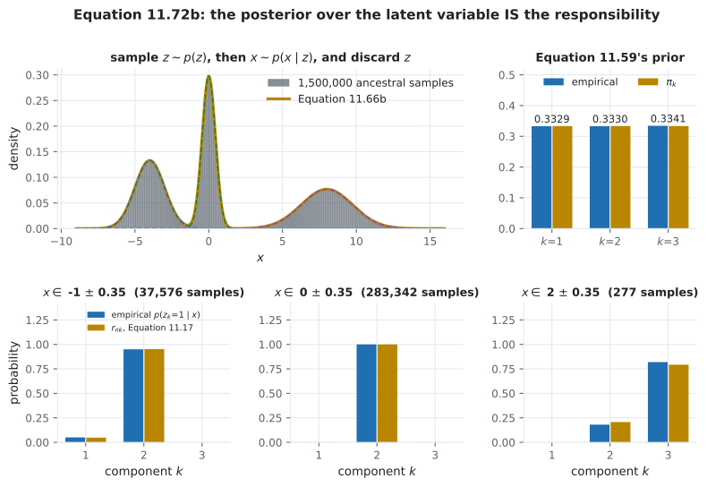
Ancestral sampling, run $1.5$ million times: the samples reproduce Equation 11.66b to $3.4\times10^{-4}$ in bin probability, against a sampling floor of $1.7\times10^{-4}$ .
Equation 11.72b: the responsibility is a posterior. Computed the long way — joint over marginal — it matches Equation 11.17 to $\mathbf{0.0}$ , and the empirical posterior from labelled samples matches it too.
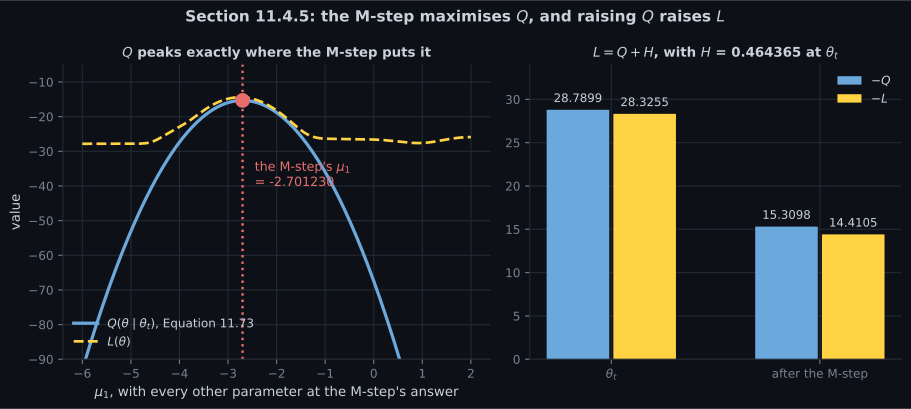
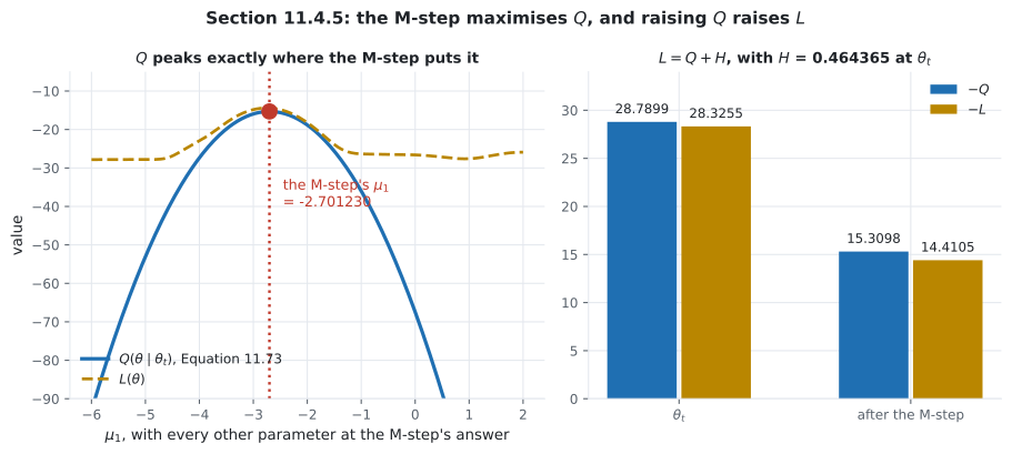
Equation 11.73’s $Q(\boldsymbol\theta\mid\boldsymbol\theta^{(t)})$ , and §11.4.5’s claim that the M-step maximises it — verified against a $40$ -restart numerical search: $5.3\times10^{-15}$ , with every parameter agreeing to six decimals.
The decomposition $L = Q + H$ , tight at $\boldsymbol\theta^{(t)}$ to $1.1\times10^{-14}$ , which is why raising $Q$ raises $L$ .
And the one thing the generative story buys that the algebra could not: data. Generate from a known mixture, refit, and watch the errors fall — $\mu$ from $0.231441$ to $0.022924$ as $N$ goes from $200$ to $200{,}000$ .

Intuition: the missing column

Imagine the dataset had one more column: which component produced each point. Fitting would be trivial — split by that column and use Chapter 8’s closed forms. The column exists; you just cannot see it.

That is the whole content of §11.4. $\mathbf{z}_n$ is the missing entry, one-hot over $K$ values. Everything the previous sections invented — the responsibilities, the weighted averages, the alternation — is what you get by writing down that model and applying Bayes’ theorem. The responsibility stops being a useful weight and becomes the posterior over the missing column.

diagram Section 11.4's model, and what each piece was called earlier mermaid

  flowchart TD
  Z["z one-hot in R^K
p(z) = pi, Equation 11.59"] -->|"p(x | z_k = 1) = N(x | mu_k, Sigma_k)
Equation 11.58"| XX["x"]
  Z --> J["joint p(x, z_k=1) = pi_k N(...)
Equation 11.61"]
  XX --> J
  J -->|"sum over z"| MARG["p(x) = sum_k pi_k N(...)
Equation 11.66b = the GMM"]
  J -->|"Bayes"| POST["p(z_k = 1 | x) = r_nk
Equation 11.72b = Equation 11.17"]
  POST --> Q["Q = E[log p(x, z | theta)]
Equation 11.73"]
  Q -->|"maximise"| MSTEP["the M-step
Equations 11.54 to 11.56"]

§11.4.1 The generative process

A binary indicator $z_k \in \{0,1\}$ says whether component $k$ made the point:

p(\mathbf{x}\mid z_k = 1) = \mathcal{N}(\mathbf{x}\mid\boldsymbol\mu_k,\boldsymbol\Sigma_k) \qquad \text{(11.58)}

$\mathbf{z} = [z_1,\ldots,z_K]^\top$ has $K-1$ zeros and exactly one $1$ — a one-hot encoding. Since the indicators are not observed, they get a prior:

p(\mathbf{z}) = \boldsymbol\pi = [\pi_1,\ldots,\pi_K]^\top, \qquad \pi_k = p(z_k = 1) \qquad \text{(11.59), (11.60)}

and the joint follows:

p(\mathbf{x}, z_k = 1) = p(\mathbf{x}\mid z_k = 1)p(z_k = 1) = \pi_k\mathcal{N}(\mathbf{x}\mid\boldsymbol\mu_k,\boldsymbol\Sigma_k) \qquad \text{(11.61)}

Ancestral sampling — sample $\mathbf{z}$ , then $\mathbf{x}$ given it, then throw $\mathbf{z}$ away — gives “valid samples from the GMM”. Run $1.5$ million times:

	value
empirical mean	$1.336079$ against a theoretical $1.333333$
empirical variance	$26.296641$ against $26.288889$
largest gap in bin probability, $120$ bins	$3.367\times10^{-4}$
total variation distance	$0.002549$
sampling floor, $\sqrt{p_{\max}/M}$	$1.696\times10^{-4}$

Top left, a grey histogram with three humps under a yellow curve that traces it exactly. Top right, three pairs of near-identical bars around one third. Bottom, three pairs of bar charts, each pair matching closely. — The samples never see Equation 11.66b — they come from drawing a component and then a point from it. The bottom row is Equation 11.72b checked empirically: take every sample that landed near a given x, look up which component actually produced it, and the proportions are the responsibilities.

§11.4.3 The responsibility is a posterior

Bayes’ theorem on the joint:

p(z_k = 1\mid\mathbf{x}) = \frac{p(z_k = 1)p(\mathbf{x}\mid z_k = 1)}{\sum_j p(z_j = 1)p(\mathbf{x}\mid z_j = 1)} = \frac{\pi_k\mathcal{N}(\mathbf{x}\mid\boldsymbol\mu_k,\boldsymbol\Sigma_k)}{\sum_j\pi_j\mathcal{N}(\mathbf{x}\mid\boldsymbol\mu_j,\boldsymbol\Sigma_j)} \qquad \text{(11.69)}

which we identify as the responsibility of the $k$ th mixture component for data point $\mathbf{x}$ .

Computed the long way on the book’s seven points — form the joint of Equation 11.61, divide by the marginal of Equation 11.66b — against page 1103’s Equation 11.17:

	value
$\max\lvert p(z_{nk}=1\mid\mathbf{x}_n) - r_{nk}\rvert$	$\mathbf{0.0}$

Not approximately. The same arithmetic, written twice, three sections apart.

§11.2.1 could only say the responsibility was “a soft assignment” and that $\mathbf{r}_n$ was “a normalized probability vector” — true, but with nothing behind it. Now it has a referent: $r_{nk}$ is the probability that component $k$ did in fact generate $\mathbf{x}_n$ , under a model that says one of them did.

That is what licenses three things the earlier sections did without justification:

Summing responsibilities as if they were counts. $N_k = \sum_n r_{nk}$ is the expected number of points component $k$ generated, which is why page 1104’s $\mu_k$ is a legitimate estimator and page 1106’s $\pi_k = N_k/N$ is a legitimate proportion.

Treating the soft assignment as differentiable. A posterior is a smooth function of the parameters; a hard assignment is not.

Alternating at all. Which is §11.4.5, below.

§11.4.5 The M-step maximises Q

Given the current parameters $\boldsymbol\theta^{(t)}$ , the E-step computes

Q(\boldsymbol\theta\mid\boldsymbol\theta^{(t)}) = \mathbb{E}_{\mathbf{z}\mid\mathbf{x},\boldsymbol\theta^{(t)}}\left[\log p(\mathbf{x},\mathbf{z}\mid\boldsymbol\theta)\right] \qquad \text{(11.73a)}

and “the M-step selects an updated set of model parameters $\boldsymbol\theta^{(t+1)}$ by maximizing” it. The book states this and stops. Checked, on the book’s own initialisation:

	$Q$
at the M-step’s answer (Equations 11.54–11.56)	$-15.3098303659$
at a $40$ -restart Nelder–Mead maximum of $Q$	$-15.3098303659$
difference	$\mathbf{+5.3\times10^{-15}}$

and parameter by parameter:

	optimiser	the M-step
$\boldsymbol\pi$	$0.287001,\ 0.293890,\ 0.419109$	$0.287001,\ 0.293890,\ 0.419109$
$\boldsymbol\mu$	$-2.701230,\ -0.403411,\ 3.704287$	$-2.701230,\ -0.403411,\ 3.704287$
$\boldsymbol\sigma^2$	$0.144000,\ 0.438492,\ 1.526594$	$0.144000,\ 0.438492,\ 1.526594$

Left, a blue parabola-like curve peaking at a marked red point where a dashed yellow curve touches it. Right, four bars in two groups, the blue slightly taller than the yellow in each. — On the left, Q as a function of the first mean with everything else held at the M-step's answer; the red marker is where Equations 11.54 to 11.56 put it, and it is the peak. The dashed curve is the actual log-likelihood, which touches Q at that point and is larger everywhere else.

Write $H(\mathbf{r}) = -\sum_{n,k} r_{nk}\log r_{nk}$ , the entropy of the responsibilities. Then

L(\boldsymbol\theta^{(t)}) = Q(\boldsymbol\theta^{(t)}\mid\boldsymbol\theta^{(t)}) + H(\mathbf{r})

Measured at the book’s initialisation:

	value
$L(\boldsymbol\theta^{(t)})$	$-28.3255356559$
$Q(\boldsymbol\theta^{(t)}\mid\boldsymbol\theta^{(t)})$	$-28.7899007529$
$H(\mathbf{r})$	$0.4643650970$
$Q + H$	$-28.3255356559$
gap	$\mathbf{1.1\times10^{-14}}$

Since $H \geq 0$ , $Q$ is a lower bound on $L$ — and at $\boldsymbol\theta = \boldsymbol\theta^{(t)}$ the bound is tight. So maximising $Q$ cannot lower $L$ : you push up a bound that touches the thing you care about. Page 1107’s $180{,}000$ -step measurement is this identity, observed.

And the bound is loose in a useful direction. After the M-step:

	rose by
$Q$	$+13.480070$
$L$	$\mathbf{+13.915050}$

$L$ rose by more than $Q$ did, because the responsibilities at the new parameters are more confident, so the next entropy term is larger. EM gets the bound’s improvement plus the slack.

What the story buys that the algebra could not

Generate data from a known mixture — $\boldsymbol\pi = (0.5, 0.2, 0.3)$ , $\boldsymbol\mu = (-2, 1, 4)$ , $\boldsymbol\sigma^2 = (0.5, 2, 1)$ — and fit it back, best of five restarts:

$N$	$\max\lvert\boldsymbol\mu - \text{truth}\rvert$	$\max\lvert\boldsymbol\sigma^2 - \text{truth}\rvert$	$\max\lvert\boldsymbol\pi - \text{truth}\rvert$
$200$	$0.231441$	$1.605373$	$0.060564$
$2000$	$0.361082$	$1.052217$	$0.045084$
$20{,}000$	$0.068719$	$0.556054$	$0.036519$
$200{,}000$	$\mathbf{0.022924}$	$\mathbf{0.080283}$	$\mathbf{0.005596}$

Each row is a single dataset, so individual rows fluctuate — the $N = 2000$ draw is unlucky on the means. Across the three orders of magnitude the trend is unambiguous: $\mu$ improves by $10\times$ , $\sigma^2$ by $20\times$ , $\boldsymbol\pi$ by $11\times$ , against the $\sqrt{1000} \approx 31.6$ a perfectly behaved estimator would give.

This check is only possible because of §11.4. Without a generative process there is no “truth” to recover — you can measure a likelihood, but you cannot ask whether the parameters are right.

pch.quizTag Does the latent-variable view land?

What is the latent variable z in Section 11.4?

pch.quizShowAnswer

B — A one-hot indicator saying which of the K components generated the point — Chapter 10's latent variable was continuous and lived in R^M; this one is discrete with K states. Think of it as a missing column in the dataset: if you could see which component made each point, fitting would be Chapter 8's closed forms applied group by group.
What is the relationship between the responsibility and the posterior over z?

pch.quizShowAnswer

B — They are the same quantity — computing the joint over the marginal reproduces Equation 11.17 to exactly 0.0 — Section 11.2.1 could only call the responsibility a soft assignment. Now it has a referent: the probability that component k did in fact generate the point. That is what licenses treating the column sums as counts, and what makes the assignment differentiable.
Does the M-step really maximise Q, or is that an approximation?

pch.quizShowAnswer

B — It is exact — a 40-restart numerical maximisation of Q lands on the same parameters to six decimals, differing in Q by 5.3e-15 — Every parameter agrees: the weights, the means and the variances. The three weighted averages of Section 11.2 are not a heuristic that happens to work — they are the closed-form argmax of the expected complete-data log-likelihood.
Why does raising Q raise L?

pch.quizShowAnswer

B — Because L = Q + H with H the entropy of the responsibilities, so Q is a lower bound on L that is tight at the current parameters — Measured at the book's initialisation: Q is minus 28.7899, H is 0.4644, and their sum is L to 1.1e-14. After the M-step, Q rose by 13.480070 and L by 13.915050 — L gains more, because the new responsibilities are more confident and the entropy term grows too.

Exercises

Exercise 1 – Sample from the story, recover the density

Exercise 2 – The responsibility, computed as a posterior

Exercise 3 – Does the M-step maximise Q?

Exercise 4 – L equals Q plus an entropy

Exercise 5 – Generate, then recover

Recall card

Section 11.4 adds a missing column to the dataset: a one-hot indicator saying which component made each point. If you could see it, fitting would be Chapter 8’s closed forms group by group.
Chapter 10’s latent variable was continuous; this one is discrete with K states, and the prior over it is the mixture weights.
Ancestral sampling from the model reproduces the mixture density — 1.5 million draws matching Equation 11.66b to a bin-probability gap of 3.4e-04, against a sampling floor of 1.7e-04.
The responsibility is a posterior, exactly. Computing the joint over the marginal reproduces Equation 11.17 to 0.0, not approximately.
That is what licenses three earlier moves: summing responsibilities as counts, differentiating a soft assignment, and alternating at all.
The M-step is the exact argmax of Q, the expected complete-data log-likelihood — matched by a forty-restart numerical search to 5.3e-15, with every parameter agreeing to six decimals.
So the three weighted averages of Section 11.2 are not heuristics. They are a closed-form maximisation of something.
L equals Q plus the entropy of the responsibilities, measured to 1.1e-14, so Q is a lower bound that is tight at the current parameters.
Raising a tight lower bound cannot lower what it bounds, which is page 1107’s monotonicity guarantee with a reason attached.
And L rises by more than Q does — 13.915050 against 13.480070 — because the new responsibilities are sharper, so the entropy grows too.
The generative story also supplies a truth to recover. Fitting data generated from known parameters, the errors fall by factors of 10, 20 and 11 as N goes from 200 to 200,000.
Without Section 11.4 that check does not exist: you can measure a likelihood, but you cannot ask whether the parameters are right.

Next: Chapter 11 Worked Problems — problems built from the chapter’s own claims, this module’s own.

pch.coffeeTagline

pch.coffeeCta

pch.feedbackHeading

pch.feedbackSubheading