What you’ll learn

• the bootstrap, and the derivation of the 63.2% / 36.8% split
• out-of-bag scoring — a validation estimate that costs nothing
• bagging against pasting, and why the resampling that seems wasteful wins
• what a random forest adds beyond bagging, and why it lowers correlation
• Extra-Trees, which makes each tree worse and the ensemble better
• why feature_importances_feature_importances_ favours high-cardinality columns, measured

Intuition

The Power of Ensembles established that averaging cancels variance only when the members disagree. Bagging manufactures that disagreement mechanically: train each model on a different random sample of the same data.

A deep decision tree is the ideal member. It has low bias, catastrophic variance, and — because the greedy split search amplifies small differences — two trees grown on slightly different samples can look nothing alike. High variance and low correlation are exactly what averaging needs.

  flowchart TD
  D["Training set, n rows"] --> B1["bootstrap 1
n rows, with replacement"]
  D --> B2["bootstrap 2"]
  D --> B3["bootstrap ..."]
  B1 --> T1["deep tree 1"]
  B2 --> T2["deep tree 2"]
  B3 --> T3["deep tree m"]
  T1 --> A["Average (regression)
or vote (classification)"]
  T2 --> A
  T3 --> A

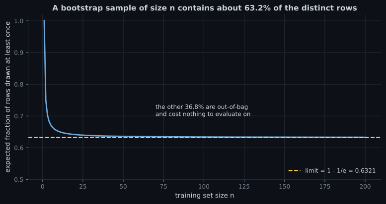
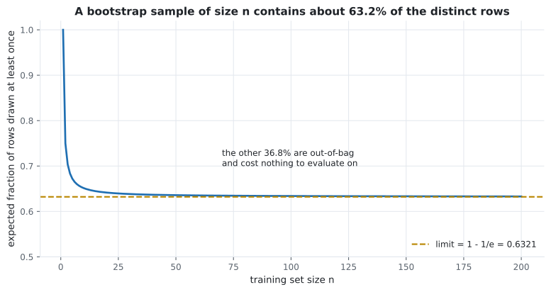
The math: what a bootstrap sample contains

Draw $n$ rows with replacement from a set of $n$. For any particular row, the chance of not being picked on one draw is $1 - 1/n$, and the draws are independent:

As $n$ grows this converges to a familiar constant:

figureCoverage converges almost immediatelymatplotlib

Each tree therefore misses about a third of the data — and those rows are a ready-made validation set for that tree, at no extra cost.

See it move

Twenty rows, drawn with replacement twenty times. Watch which rows get picked more than once and which are left out entirely — the leftovers are that tree’s out-of-bag set.

Out-of-bag scoring

For each training row, average the predictions of only those trees that never saw it. That is a genuine held-out estimate, computed during training, using data you already paid for.

from sklearn.datasets import make_moons
from sklearn.ensemble import RandomForestClassifier
from sklearn.model_selection import train_test_split
 
X, y = make_moons(n_samples=800, noise=0.32, random_state=4)
X_tr, X_te, y_tr, y_te = train_test_split(X, y, test_size=0.3, random_state=0)
 
for n in (10, 100, 400):
    forest = RandomForestClassifier(n_estimators=n, oob_score=True,
                                    random_state=0, n_jobs=-1).fit(X_tr, y_tr)
    print(f"n={n:<4} oob {forest.oob_score_:.4f}   held-out test {forest.score(X_te, y_te):.4f}")
 
# n=10   oob 0.8482   held-out test 0.9250
# n=100  oob 0.8857   held-out test 0.9333
# n=400  oob 0.8946   held-out test 0.9292

from sklearn.datasets import make_moons
from sklearn.ensemble import RandomForestClassifier
from sklearn.model_selection import train_test_split
 
X, y = make_moons(n_samples=800, noise=0.32, random_state=4)
X_tr, X_te, y_tr, y_te = train_test_split(X, y, test_size=0.3, random_state=0)
 
for n in (10, 100, 400):
    forest = RandomForestClassifier(n_estimators=n, oob_score=True,
                                    random_state=0, n_jobs=-1).fit(X_tr, y_tr)
    print(f"n={n:<4} oob {forest.oob_score_:.4f}   held-out test {forest.score(X_te, y_te):.4f}")
 
# n=10   oob 0.8482   held-out test 0.9250
# n=100  oob 0.8857   held-out test 0.9333
# n=400  oob 0.8946   held-out test 0.9292

Two honest observations:

• OOB is systematically pessimistic, by 3 to 4 points here. Each row is scored by only the ~37% of trees that excluded it, so the effective ensemble is a third the size.
• The pessimism shrinks as trees are added, from 7.7 points at $n = 10$ to 3.5 at $n = 400$. At 10 trees only about 4 vote on each row, which is not an ensemble.

Use OOB for quick iteration on large data where cross-validation is expensive. Use cross-validation for the number you report.

Bagging against pasting

Bagging samples with replacement; pasting samples without. Pasting sounds cleaner — no duplicated rows — and it loses:

from sklearn.ensemble import BaggingClassifier
from sklearn.tree import DecisionTreeClassifier
 
bagging = BaggingClassifier(DecisionTreeClassifier(), n_estimators=100,
                            bootstrap=True, oob_score=True,
                            random_state=0, n_jobs=-1).fit(X_tr, y_tr)
pasting = BaggingClassifier(DecisionTreeClassifier(), n_estimators=100,
                            bootstrap=False,
                            random_state=0, n_jobs=-1).fit(X_tr, y_tr)
 
print(f"bagging  test {bagging.score(X_te, y_te):.4f}   oob {bagging.oob_score_:.4f}")
print(f"pasting  test {pasting.score(X_te, y_te):.4f}")
 
# bagging  test 0.9417   oob 0.8786
# pasting  test 0.8833

from sklearn.ensemble import BaggingClassifier
from sklearn.tree import DecisionTreeClassifier
 
bagging = BaggingClassifier(DecisionTreeClassifier(), n_estimators=100,
                            bootstrap=True, oob_score=True,
                            random_state=0, n_jobs=-1).fit(X_tr, y_tr)
pasting = BaggingClassifier(DecisionTreeClassifier(), n_estimators=100,
                            bootstrap=False,
                            random_state=0, n_jobs=-1).fit(X_tr, y_tr)
 
print(f"bagging  test {bagging.score(X_te, y_te):.4f}   oob {bagging.oob_score_:.4f}")
print(f"pasting  test {pasting.score(X_te, y_te):.4f}")
 
# bagging  test 0.9417   oob 0.8786
# pasting  test 0.8833

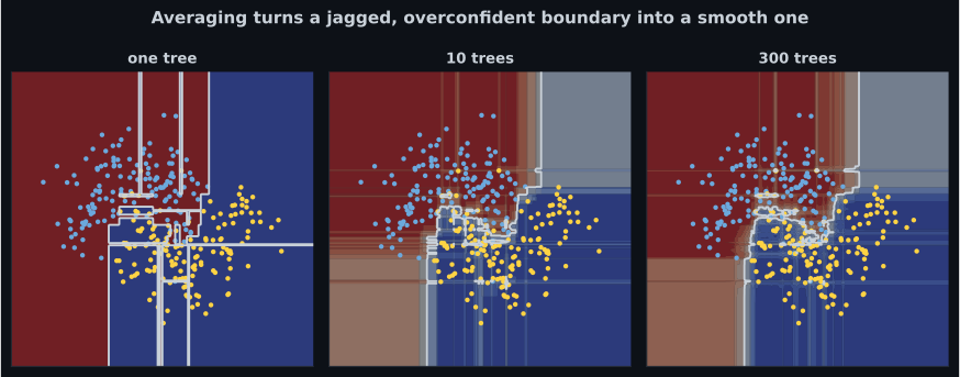
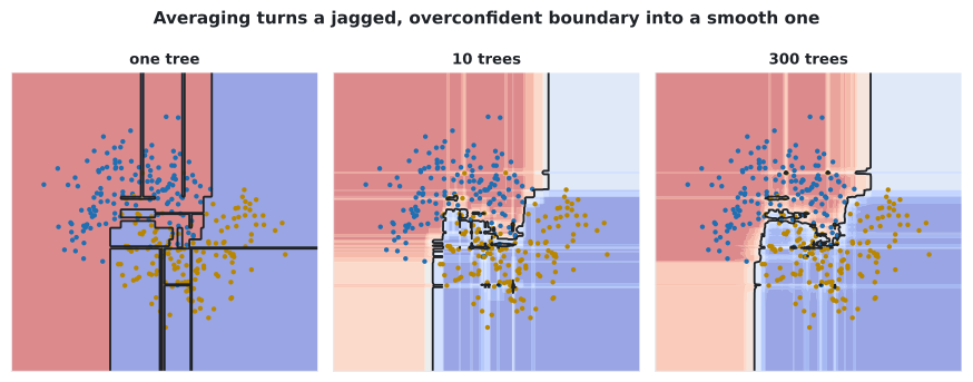
Bagging wins by 5.8 points. The reason is the correlation term from the previous page: sampling with replacement makes the training sets more different from each other, so $\rho$ falls. Each individual tree is slightly worse — it has seen only 63% of the distinct rows — and the ensemble is much better. Duplicated rows are a feature.

Pasting without replacement on 100 estimators reuses nearly the same rows every time, so the trees are near-identical and averaging them accomplishes little.

What a random forest adds

Bagging alone leaves a problem. If one feature is strongly predictive, every tree will split on it first, whatever rows it received. The trees stay correlated through the feature, not the data.

A random forest fixes this by sampling features at each split, not just rows:

With $\sqrt{n}$ features considered per split, the dominant feature is unavailable for most splits, forcing trees to find alternative structure. Individual trees get worse; $\rho$ drops; the ensemble improves.

figureOne tree, ten trees, three hundredmatplotlib

figureWhere adding trees stops payingmatplotlib

Reading the plot

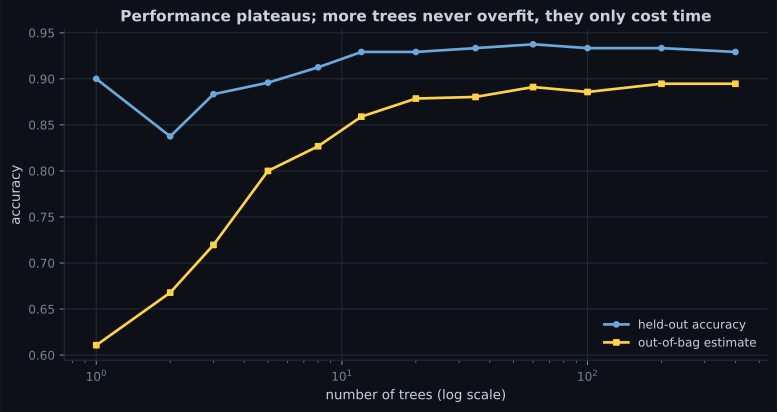
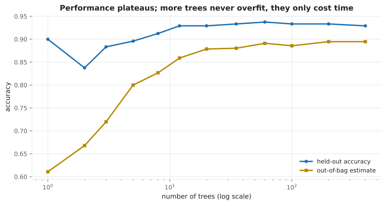
1. n_estimatorsn_estimators is not a regularisation parameter. Adding trees cannot overfit; each is an independent draw and the average converges. Anything else in this curriculum with “more” on the dial eventually turns against you.
2. The plateau arrives quickly. By 60 trees the curve is flat. Going 100 → 400 changed held-out accuracy from 0.9333 to 0.9292 — noise, not improvement.
3. OOB tracks the test curve in shape, sitting a few points below. Useful for choosing n_estimatorsn_estimators even though its level is pessimistic.

Set n_estimatorsn_estimators as high as your latency budget allows, then tune the parameters that actually trade off — max_depthmax_depth, min_samples_leafmin_samples_leaf, max_featuresmax_features.

Extra-Trees

Extremely Randomised Trees go one step further: instead of searching for the best threshold on each sampled feature, they pick thresholds at random and keep the best of those.

Measured on the same split: random forest 0.9333, Extra-Trees 0.9375. Deliberately worse members, a better ensemble, and faster to train. It is worth trying whenever a forest is your baseline.

Feature importance lies

figureFour features: two informative, two pure noisematplotlib

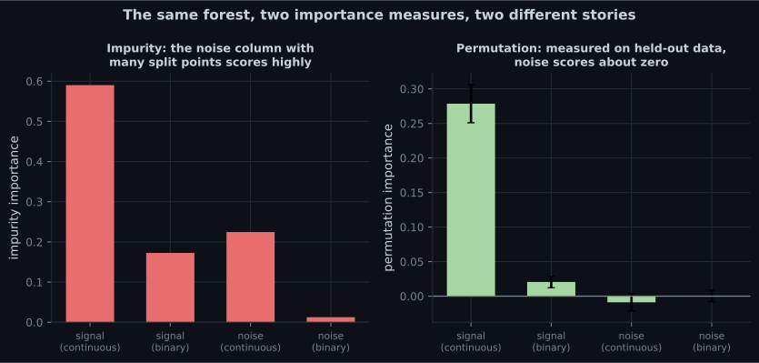
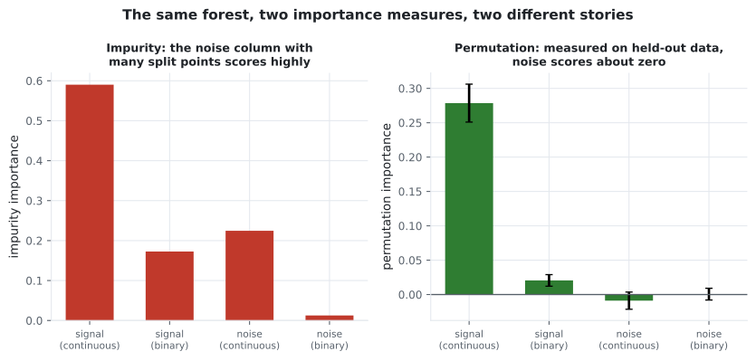
Measured on a constructed dataset where two columns carry signal and two are pure noise:

Impurity importance ranks a pure-noise column second, above a genuinely informative one. The mechanism is mechanical: a continuous feature offers hundreds of candidate split points, a binary feature offers exactly one. More chances to win a split by luck means more accumulated impurity reduction.

Permutation importance shuffles one column in the held-out data and measures how much the score drops. Noise scores zero because destroying noise costs nothing.

from sklearn.inspection import permutation_importance
 
result = permutation_importance(forest, X_test, y_test,
                                n_repeats=15, random_state=0, n_jobs=-1)
 
for name, mean, std in sorted(zip(names, result.importances_mean,
                                  result.importances_std),
                              key=lambda row: -row[1]):
    print(f"{name:<14} {mean:+.4f} +/- {std:.4f}")

from sklearn.inspection import permutation_importance
 
result = permutation_importance(forest, X_test, y_test,
                                n_repeats=15, random_state=0, n_jobs=-1)
 
for name, mean, std in sorted(zip(names, result.importances_mean,
                                  result.importances_std),
                              key=lambda row: -row[1]):
    print(f"{name:<14} {mean:+.4f} +/- {std:.4f}")

Pitfalls

Compare

The “trains in parallel” column is the practical difference between this page and the next two. Bagging is embarrassingly parallel; boosting is inherently sequential.

🧪 Try It Yourself

Exercise 1 – Derive the 63.2%

Exercise 2 – Free validation with out-of-bag scoring

Exercise 3 – Bagging against pasting

Exercise 4 – Extra-Trees against a forest

Exercise 5 – Catch impurity importance lying

Recap

• A bootstrap sample of size $n$ contains $1 - (1-1/n)^n \to 63.2\%$ of the distinct rows; the remaining 36.8% is the out-of-bag set.
• OOB scoring is free and systematically pessimistic — 0.8857 against a true 0.9333 at 100 trees.
• Bagging beat pasting 0.9417 to 0.8833, because replacement lowers the correlation between trees.
• A random forest samples features at every split, so no single dominant feature can keep the trees correlated.
• Extra-Trees randomises thresholds too: worse trees, lower correlation, better ensemble (0.9375), faster training.
• n_estimatorsn_estimators cannot overfit — set it by your latency budget, and tune max_featuresmax_features and min_samples_leafmin_samples_leaf instead.
• Impurity importance ranked pure noise second. Use permutation importance on held-out data.

Exercise 6 – How much of the data does one tree see?

Next

Continue to Boosting - Introduction to AdaBoost — the opposite strategy: instead of averaging strong models trained in parallel, chain weak ones sequentially so each fixes the last one’s mistakes.