
K-Nearest Neighbors (KNN)
What you’ll learn
Section titled “What you’ll learn”- how a model with no training step still makes predictions
- Euclidean, Manhattan and Minkowski distance, and when the choice matters
- a full prediction worked by hand on six points — where each gives a different answer
- why is a bias-variance dial, and how to pick it
- why unscaled features destroy KNN more completely than any other model
- the curse of dimensionality, measured rather than asserted
Intuition
Section titled “Intuition”Every other model in this phase compresses the training data into parameters and then discards the data. KNN does the opposite: it stores everything and does all its work at prediction time. Asked to classify a new point, it finds the closest training points and takes a vote.
That makes it a lazy learner — fit() is essentially a memory copy — and it inverts the usual
cost profile. Training is instant; prediction is expensive, and gets more expensive as the dataset
grows.
  flowchart LR
  Q["New point q"] --> D["Distance from q
to every training point"]
  D --> S["Sort, keep the k smallest"]
  S --> V["Majority vote among those k"]
  V --> P["Predicted class"]
  S --> R["Vote proportions
= predicted probabilities"]
The math
Section titled “The math”Distance
Section titled “Distance”The default is Euclidean distance, the straight line between two points:
It is one case of the Minkowski family, parameterised by :
| Name | Behaviour | |
|---|---|---|
| 1 | Manhattan | Sum of axis-wise distances; robust to one wild coordinate |
| 2 | Euclidean | Straight line; the default |
| Chebyshev | The single largest coordinate difference |
scikit-learn exposes this as metric="minkowski", p=2. On high-dimensional data often
works better, because Euclidean distances concentrate — see the measurement below.
The prediction rule
Section titled “The prediction rule”where is the set of indices of the closest training points. The class proportions inside that set are the predicted probabilities — which is why KNN probabilities come in steps of and are coarse for small .
With weights="distance" each neighbour instead votes with weight , so closer points count
for more and exact ties become rare.
Worked example by hand
Section titled “Worked example by hand”Six training points, two features, two classes. Classify the query .
| point | class | |||||
|---|---|---|---|---|---|---|
| A | 1 | 1 | 0 | −3 | −3 | |
| B | 2 | 2 | 0 | −2 | −2 | |
| C | 3 | 3 | 0 | −1 | −1 | |
| D | 4 | 5 | 1 | 0 | +1 | |
| E | 6 | 5 | 1 | +2 | +1 | |
| F | 7 | 7 | 1 | +3 | +3 |
Step 1 — rank by distance.
Step 2 — vote, for three values of .
| Neighbours | Votes | Prediction | ||
|---|---|---|---|---|
| 1 | D | 1 → class 1 | 1 | 1.00 |
| 3 | D, C, E | 2 → class 1, 1 → class 0 | 1 | 0.67 |
| 5 | D, C, E, B, A | 2 → class 1, 3 → class 0 | 0 | 0.40 |
The same query, the same data, and flips the answer. With the nearest point decides everything; by the vote has reached back into the cluster of class-0 points and reversed the verdict. This is not a pathological example — it is ordinary behaviour near a boundary, and it is exactly why must be cross-validated rather than guessed.
Choosing k
Section titled “Choosing k”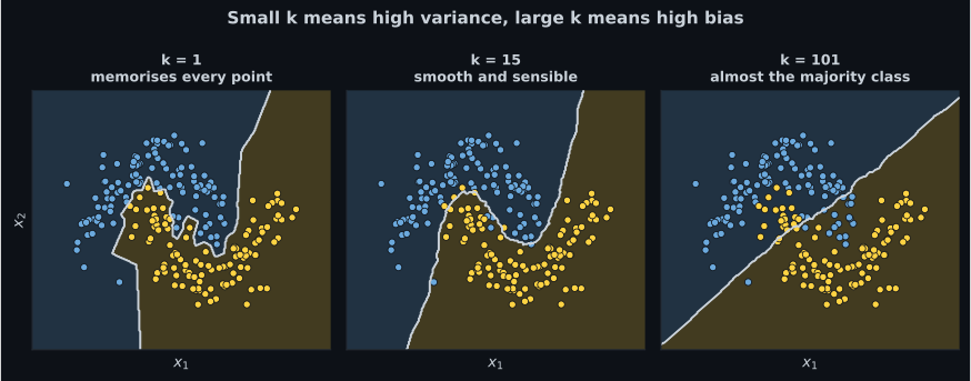
Reading the plot
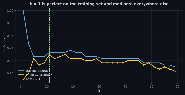
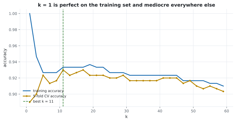
Section titled “Reading the plot”- Training accuracy at is always exactly 1.0. Each point retrieves itself, at distance zero. This is the cleanest demonstration in the curriculum that a training score can be structurally meaningless.
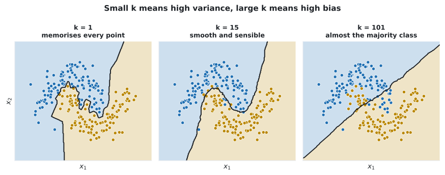
- The CV curve peaks and then declines. Small is high variance, large is high bias, and the peak is the trade.
- The peak is broad. Anything from roughly 7 to 21 performs within noise of the best here. Choose from the middle of the plateau rather than the exact argmax.
Two rules of thumb, neither of which replaces cross-validation:
- Use an odd for binary problems so a majority always exists.
- is a reasonable starting point ( here).
See it move
Section titled “See it move”Move the mouse to place a query point. The sketch draws a circle out to its -th nearest neighbour, connects the voting neighbours, and tallies the vote — so you can see the prediction change as the circle swallows one more point. The background is the full decision boundary at the current , recomputed on a grid.
Three things become obvious by moving rather than reading. At the background is full of
single-point islands — each one is a noisy label that owns its own territory. At the
boundary is nearly straight and the crescents are gone, because a 61-neighbour vote over 90 points
is averaging two thirds of the dataset into every prediction. And near the boundary at any , the vote margin drops to one or two, which is the
honest signal that the model has no opinion there — a probability KNN can report as
predict_proba and that a threshold decision should respect.
Scaling is not optional
Section titled “Scaling is not optional”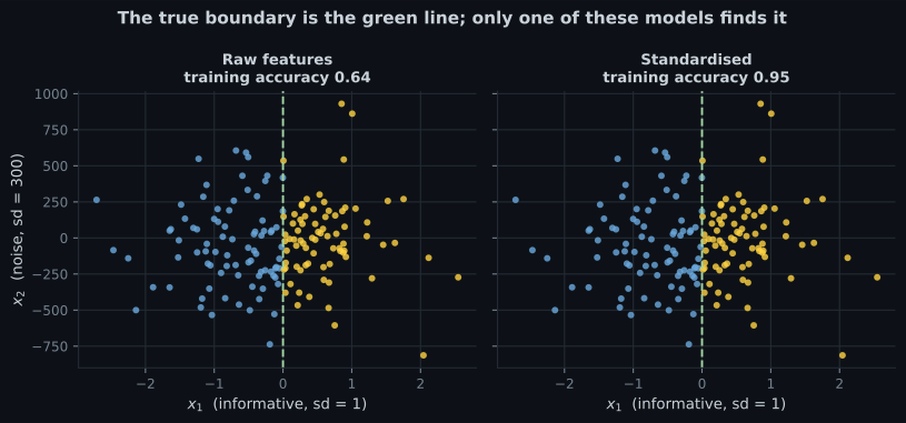
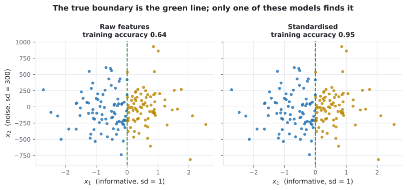
The reason is arithmetic. In , a feature with a range of 300 contributes terms 90,000 times larger than one with a range of 1. The small feature is not down-weighted — it is erased.
Every other model can compensate by learning a larger coefficient. KNN has no coefficients, which makes it the model most sensitive to scaling in the entire curriculum.
from sklearn.datasets import load_breast_cancer
from sklearn.model_selection import train_test_split
from sklearn.neighbors import KNeighborsClassifier
from sklearn.pipeline import make_pipeline
from sklearn.preprocessing import StandardScaler

X, y = load_breast_cancer(return_X_y=True)
y = 1 - y
X_tr, X_te, y_tr, y_te = train_test_split(
    X, y, test_size=0.3, random_state=0, stratify=y
)

for k in (1, 5, 15):
    raw = KNeighborsClassifier(k).fit(X_tr, y_tr).score(X_te, y_te)
    scaled = make_pipeline(
        StandardScaler(), KNeighborsClassifier(k)
    ).fit(X_tr, y_tr).score(X_te, y_te)
    print(f"k={k:<3} raw {raw:.4f}   scaled {scaled:.4f}")

# k=1   raw 0.9123   scaled 0.9298
# k=5   raw 0.9357   scaled 0.9415
# k=15  raw 0.9357   scaled 0.9474
Scaling gains one to two points at every here, because the breast-cancer features already sit within a couple of orders of magnitude of each other. With genuinely mismatched units — age in years beside income in currency — the gap is far larger.
From scratch
Section titled “From scratch”import numpy as np
from collections import Counter
def knn_predict(X_train, y_train, query, k=3):
"""Distances, sort, vote. That is the entire algorithm."""
distances = np.linalg.norm(X_train - query, axis=1)
nearest = np.argsort(distances)[:k]
votes = Counter(y_train[nearest])
winner, count = votes.most_common(1)[0]
return winner, count / k, distances[nearest]
X = np.array([[1.0, 1], [2, 2], [3, 3], [4, 5], [6, 5], [7, 7]])
y = np.array([0, 0, 0, 1, 1, 1])
q = np.array([4.0, 4])
for k in (1, 3, 5):
label, confidence, dists = knn_predict(X, y, q, k)
print(f"k={k}: class {label} confidence {confidence:.2f} "
f"distances {dists.round(3)}")
# k=1: class 1 confidence 1.00 distances [1.]
# k=3: class 1 confidence 0.67 distances [1. 1.414 2.236]
# k=5: class 0 confidence 0.60 distances [1. 1.414 2.236 2.828 4.243]At the confidence 0.60 refers to the winning class 0, so the probability of class 1 is 0.40 — matching the hand-worked table.
The curse of dimensionality
Section titled “The curse of dimensionality”KNN rests on one assumption: that “nearby” means “similar”. In high dimensions that assumption quietly fails.
Take 1,000 points spread uniformly through a unit hypercube and measure how far the nearest and the farthest are from a query point. As dimensions grow, those two numbers converge:
import numpy as np

rng = np.random.default_rng(0)

print(f"{'dims':>5} {'nearest':>9} {'farthest':>9} {'ratio':>7}")
for n_dims in (2, 10, 100, 1000):
    X = rng.random((1000, n_dims))
    q = rng.random(n_dims)
    d = np.linalg.norm(X - q, axis=1)
    print(f"{n_dims:>5} {d.min():>9.3f} {d.max():>9.3f} {d.max() / d.min():>7.2f}")

#  dims   nearest  farthest   ratio
#     2     0.010     1.334  135.62
#    10     0.471     2.111    4.48
#   100     3.349     4.653    1.39
#  1000    12.166    13.553    1.11
In two dimensions the farthest point is 136 times further away than the nearest. In a thousand dimensions it is 11% further — “nearest” has stopped carrying information, and a vote among the five closest points is a vote among five essentially arbitrary points. Reduce dimensionality with PCA before applying KNN to wide data, or use a model that learns which features matter.
pch.algoApi sklearn.neighbors.KNeighborsClassifier
pch.algoAssumes
- Points close together in feature space tend to share a label
- All features are on comparable scales
- The feature count is low enough that distances still discriminate
- The training set is dense enough to have genuine neighbours
pch.algoCost
- pch.algoTrain
O(1) — it stores the data- pch.algoPredict
O(m·n) brute force, O(n log m) with a KD-tree- pch.algoMemory
O(m·n) — the whole training set
m = training samples, n = features
pch.algoHyperparams
-
n_neighborsdefault 5 The bias-variance dial. Small k gives jagged boundaries; large k smooths toward the majority class. -
weightsdefault uniform 'distance' weights each neighbour by 1/d, so closer points count more and ties become rare. -
metric / pdefault minkowski, p=2 p=2 is Euclidean, p=1 is Manhattan. Manhattan often holds up better in higher dimensions. -
algorithmdefault auto 'kd_tree' and 'ball_tree' speed up low-dimensional prediction; above roughly 20 features they degrade to brute force.
pch.algoReachFor
- You want a strong non-linear baseline with almost no assumptions
- The decision boundary is irregular and local
- The dataset is small to medium and prediction latency is not critical
- You need a quick check on whether the features carry signal at all
pch.algoLookElsewhere
- There are many features — distances stop discriminating
- The training set is large and predictions must be fast
- Features cannot be scaled sensibly
- You need an interpretable model; KNN offers no coefficients and no rules
Pitfalls
Section titled “Pitfalls”Compare
Section titled “Compare”| Model | Training cost | Prediction cost | Needs scaling | Boundary shape |
|---|---|---|---|---|
| KNN | None | High — | Critically | Arbitrarily local |
| Logistic Regression | Moderate | Yes, for the solver | Linear | |
| SVM (RBF) | High | Critically | Smooth, non-linear | |
| Decision Tree | Moderate | No | Axis-aligned steps | |
| Naive Bayes | Very low | No | Smooth, from densities |
KNN and decision trees make a useful first pair: both handle non-linear boundaries, and their failure modes are opposite. If both do badly, the features are probably the problem.
-
Why does KNN have a training accuracy of exactly 1.0 when k = 1?
With k = 1 the closest point to any training row is that row itself, at distance zero. The training score is structurally guaranteed and carries no information.
pch.quizShowAnswer
B — Because each training point is its own nearest neighbour, so it always retrieves its own label — With k = 1 the closest point to any training row is that row itself, at distance zero. The training score is structurally guaranteed and carries no information.
-
Why does KNN suffer more from unscaled features than logistic regression does?
Logistic regression can learn a small coefficient for a wide-ranging feature. KNN has nothing to learn: the squared difference of a feature spanning 300 units swamps one spanning 1.
pch.quizShowAnswer
B — Because it has no coefficients that could compensate — the distance metric is fixed, so a wide-ranging feature dominates it outright — Logistic regression can learn a small coefficient for a wide-ranging feature. KNN has nothing to learn: the squared difference of a feature spanning 300 units swamps one spanning 1.
-
In the worked example, k = 1 and k = 3 predict class 1 but k = 5 predicts class 0. What does that tell you?
Near a boundary the composition of the neighbourhood changes rapidly with k. This is precisely why k must be cross-validated rather than assumed.
pch.quizShowAnswer
B — The query sits near a decision boundary, where the answer depends on how far the vote reaches — Near a boundary the composition of the neighbourhood changes rapidly with k. This is precisely why k must be cross-validated rather than assumed.
-
In 1,000 dimensions the farthest of 1,000 random points is only 11% further away than the nearest. Why does that break KNN?
KNN assumes proximity implies similarity. Once all pairwise distances converge, the k nearest neighbours are no longer meaningfully closer than any other k points.
pch.quizShowAnswer
B — Because 'nearest' stops being meaningfully different from 'farthest', so the vote becomes effectively random — KNN assumes proximity implies similarity. Once all pairwise distances converge, the k nearest neighbours are no longer meaningfully closer than any other k points.
🧪 Try It Yourself
Section titled “🧪 Try It Yourself”Exercise 1 – Compute the distances
Section titled “Exercise 1 – Compute the distances”Exercise 2 – Vote by majority
Section titled “Exercise 2 – Vote by majority”Exercise 3 – Scaling changes the score
Section titled “Exercise 3 – Scaling changes the score”Exercise 4 – Cross-validate k
Section titled “Exercise 4 – Cross-validate k”Exercise 5 – Watch distances converge
Section titled “Exercise 5 – Watch distances converge”- KNN stores the training set and votes at prediction time — no parameters, no training step.
- Distance is the model. Euclidean by default, Manhattan often better in higher dimensions.
- Worked by hand: the query is class 1 at and , and class 0 at .
- Small is high variance, large is high bias; training accuracy at is always 1.0 and always meaningless.
- Scaling is mandatory — a feature with a 300-unit range erases one with a 1-unit range.
- In 1,000 dimensions the nearest and farthest points differ by 11%, and the whole premise collapses.
Exercise 6 – One query point, four values of
Section titled “Exercise 6 – One query point, four values of kkk”Continue to Support Vector Machines (SVM) — a model that keeps only the handful of points that actually define the boundary and ignores the rest.
pch.coffeeTagline
pch.coffeeCtapch.feedbackHeading
pch.feedbackSubheading