
Variational Autoencoders (VAE)
The previous page ended on a specific failure: an autoencoder’s code space has no shape, so sampling a random code and decoding it produces nothing. A VAE fixes that with two changes — the encoder outputs a distribution instead of a point, and the loss adds a term pulling those distributions towards a standard normal.
Both changes have a dial, and the dial has two failure modes at its ends. Measured on MNIST with a 2-dimensional latent:
| β (weight on KL) | Reconstruction MSE | KL (nats) | Spread of the means | Mean posterior variance | Active dimensions |
|---|---|---|---|---|---|
| 0 | 0.0433 | 183.337 | 10.6794 | 0.0001 | 2 of 2 |
| 0.5 | 0.0447 | 6.033 | 1.1980 | 0.0057 | 2 of 2 |
| 1 | 0.0450 | 5.366 | 1.0892 | 0.0104 | 2 of 2 |
| 4 | 0.0477 | 3.236 | 0.8950 | 0.0401 | 2 of 2 |
| 20 | 0.0617 | 0.318 | 0.4519 | 0.7459 | 1 of 2 |
At β = 0 it is an autoencoder with a noisy encoder and a latent 10× wider than the prior. At β = 20 the latent carries almost nothing. The useful range is narrow and the ends fail in opposite directions.
What you’ll learn
Section titled “What you’ll learn”- Why the encoder outputs a mean and a log-variance, and what the reparameterisation trick is for.
- The two loss terms, and the measured trade between them: reconstruction 0.0433 → 0.0617 as KL falls 183.337 → 0.318.
- Posterior collapse, measured: at β = 20 only 1 of 2 latent dimensions stays active and the posterior variance rises to 0.7459 (the prior’s is 1.0).
- Why β = 1 produces an aggregate posterior that actually matches the prior — mean distance from the origin 1.2674 against 1.2533 expected.
- What the latent space looks like, and why interpolation works here and not in a plain autoencoder.
Two changes to an autoencoder
Section titled “Two changes to an autoencoder”The second term is the whole difference. It penalises encoders whose output distribution strays from a standard normal, which makes the code space dense — every point near the origin decodes to something plausible, because the encoder was pushed to use exactly that region.
mean = keras.layers.Dense(latent)(x)
log_variance = keras.layers.Dense(latent)(x)

class Sampler(keras.layers.Layer):
    def call(self, inputs):
        mean, log_variance = inputs
        noise = tf.random.normal(tf.shape(mean))
        return mean + tf.exp(0.5 * log_variance) * noise      # <- reparameterisation
Sampling is not differentiable, but this form of it is: the randomness sits in noise,
which has no parameters, and the gradient flows through mean and log_variance as
ordinary tensors. That is the reparameterisation trick, and without it the encoder
could not be trained by backpropagation at all.
The KL term has a closed form for a diagonal Gaussian against a standard normal, which is why it is one line rather than a Monte-Carlo estimate:
The trade-off, measured
Section titled “The trade-off, measured”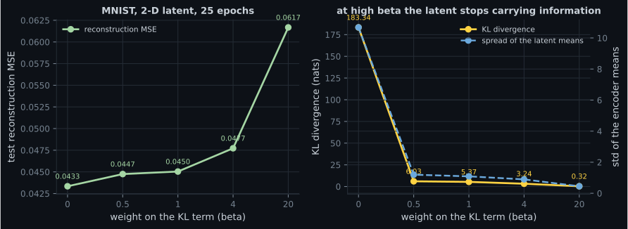
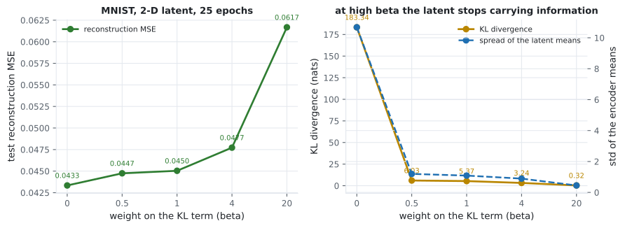
The interesting column is mean posterior variance. At β = 0 it is 0.0001 — the encoder has learned to make its distributions nearly deterministic, because noise only hurts reconstruction. As β rises, the variances grow towards the prior’s 1.0, and at β = 20 they reach 0.7459: the encoder is now emitting nearly the prior regardless of its input, which is what posterior collapse means. One of the two latent dimensions has stopped varying with the input at all.
Does the latent actually match the prior?
Section titled “Does the latent actually match the prior?”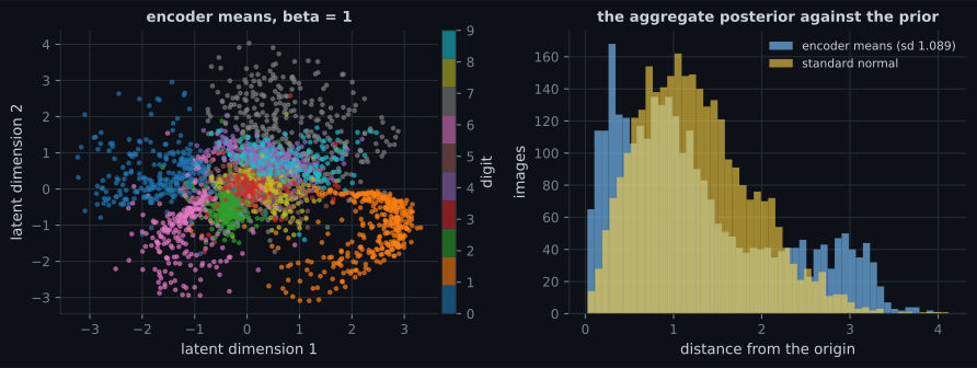
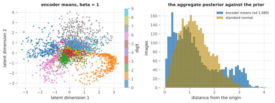
Per-digit centres from the same run show the structure the KL term buys:
| Digit | Centre | Spread |
|---|---|---|
| 1 | (+2.29, −1.05) | 1.83 |
| 0 | (−1.58, +0.42) | 1.22 |
| 7 | (+0.83, +1.69) | 1.03 |
| 6 | (−1.06, −0.88) | 0.78 |
| 3 | (+0.03, +0.04) | 0.35 |
Digits 1 and 0 — the most visually distinctive — get pushed to the edges, while 3,
5 and 8 cluster near the origin with tiny spreads, which is precisely where the
decoder’s samples are most ambiguous. A 2-dimensional latent cannot separate ten classes,
and this table shows exactly how it fails.
Sampling and interpolation
Section titled “Sampling and interpolation”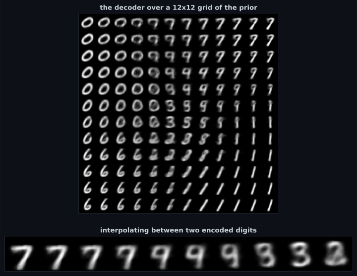
Why VAE samples are blurry
Section titled “Why VAE samples are blurry”Every VAE sample on this page is smooth, and it is not a bug in the implementation:
- The reconstruction term is a per-pixel likelihood. Its optimum is the conditional mean of all plausible images given the code, and an average of several sharp digits is a blurry digit.
- The 2-dimensional latent cannot carry enough information to disambiguate, so the conditional distribution is genuinely broad — the table above shows five digit classes sharing the region near the origin.
- The KL term further pushes codes together, which increases that overlap.
GANs replace the per-pixel likelihood with a learned discriminator and produce sharp samples instead — along with a completely different set of failure modes, measured on the next page.
  flowchart LR
  A["x"] --> B["encoder"]
  B --> C["mean"]
  B --> D["log variance"]
  C --> E["z = mean + exp(0.5·logvar)·noise"]
  D --> E
  F["noise ~ N(0, I)
no parameters"] --> E
  E --> G["decoder"]
  G --> H["reconstruction loss"]
  C -.-> I["KL towards N(0, I)"]
  D -.-> I
  I -.->|"beta = 0: KL 183.337"| J["unusable code space"]
  I -.->|"beta = 20: 1 of 2 dims active"| K["posterior collapse"]
  I -.->|"beta = 1: sd 1.0892"| L["samplable"]
Pitfalls
Section titled “Pitfalls”- Setting β = 0 and calling it a VAE. KL 183.337 and encoder means with sd 10.68 — the prior is irrelevant and sampling from it fails.
- Setting β too high. At 20 the KL fell to 0.318, one of two dimensions went inactive and reconstruction lost 0.0184 MSE.
- Not checking the aggregate posterior. The per-example KL can look fine while the combined distribution of means does not match the prior; here it did, at sd 1.0892 against 1.0.
- Sampling without the reparameterisation trick.
tf.random.normal(mean, sd)is not differentiable with respect tomean;mean + exp(0.5·logvar)·noiseis. - Expecting sharp samples from a per-pixel likelihood. Its optimum is the conditional mean, so blur is the objective working correctly.
- Using a 2-D latent for ten classes and blaming the model. Five digit classes shared the region near the origin with spreads under 0.5.
- Overriding
metricsor naming a method_lossesin a Keras 3 subclass. Both are taken; the second fails at the first training step with'TrackedList' object is not callable.
- A VAE adds a distributional encoder plus a KL term; the reparameterisation trick is what makes the sampling differentiable.
- Measured trade: reconstruction MSE 0.0433 → 0.0617 as β goes 0 → 20, with KL falling 183.337 → 0.318.
- β = 0 leaves encoder means at sd 10.68 — an autoencoder with a noisy encoder.
- β = 20 collapses the posterior: 1 of 2 dimensions active, mean posterior variance 0.7459 against the prior’s 1.0.
- At β = 1 the aggregate posterior matches the prior — mean distance 1.2674 against 1.2533 expected — which is why prior samples decode to digits.
- Samples are blurry because a per-pixel likelihood’s optimum is the conditional mean.
Replace the per-pixel likelihood with a learned discriminator and the samples get sharp — along with a new set of ways to fail: Generative Adversarial Networks (GANs).
-
What does the reparameterisation trick solve?
Sampling directly from N(mean, sd) gives no gradient path back to mean or sd, so the encoder could not be trained by backpropagation.
pch.quizShowAnswer
B — It makes sampling differentiable — writing z = mean + exp(0.5·logvar)·noise puts the randomness in a parameter-free tensor, so gradients flow through the mean and variance — Sampling directly from N(mean, sd) gives no gradient path back to mean or sd, so the encoder could not be trained by backpropagation.
-
At beta = 0 the KL divergence was 183.337 nats and the encoder means had standard deviation 10.68. What kind of model is that?
Its reconstruction is the best of the sweep (0.0433) precisely because it ignores the constraint that makes generation possible.
pch.quizShowAnswer
B — An autoencoder with a noisy encoder — nothing pulls the codes towards the prior, so sampling from the prior lands nowhere near the region the encoder uses — Its reconstruction is the best of the sweep (0.0433) precisely because it ignores the constraint that makes generation possible.
-
At beta = 20, one of two latent dimensions became inactive and the mean posterior variance rose to 0.7459. What is that called and why does it happen?
The prior's variance is 1.0, so a posterior variance approaching it means the encoder has stopped distinguishing inputs. Reconstruction rose to 0.0617 as a result.
pch.quizShowAnswer
B — Posterior collapse — the KL term dominates, so the cheapest solution is for the encoder to output the prior regardless of its input, and the latent stops carrying information — The prior's variance is 1.0, so a posterior variance approaching it means the encoder has stopped distinguishing inputs. Reconstruction rose to 0.0617 as a result.
-
Why check the aggregate posterior — the distribution of all encoder means together — rather than just the loss?
Per-example KL can be small while the aggregate distribution still has gaps or the wrong scale — and it is the aggregate that determines whether decoded prior samples look real.
pch.quizShowAnswer
B — Because prior sampling only works if the combined distribution of codes matches the prior; here mean distance from the origin was 1.2674 against 1.2533 expected for a 2-D standard normal — Per-example KL can be small while the aggregate distribution still has gaps or the wrong scale — and it is the aggregate that determines whether decoded prior samples look real.
-
Why are VAE samples blurry?
The 2-D latent makes it worse by leaving genuine ambiguity: five digit classes shared the region near the origin with spreads under 0.5.
pch.quizShowAnswer
B — A per-pixel reconstruction likelihood is optimised by the conditional mean of all plausible images for that code — and averaging several sharp digits gives a blurry one — The 2-D latent makes it worse by leaving genuine ambiguity: five digit classes shared the region near the origin with spreads under 0.5.
🧪 Try It Yourself
Section titled “🧪 Try It Yourself”pch.coffeeTagline
pch.coffeeCtapch.feedbackHeading
pch.feedbackSubheading