
Anomaly and Outlier Detection
What you’ll learn
Section titled “What you’ll learn”- the two kinds of anomaly — global and local — and why one detector cannot have both
- measured: Isolation Forest 0.9944 on global anomalies and 0.0317 on local ones
- LOF’s
n_neighborsis the whole model, and there are no labels to tune it with - what irrelevant columns do: Isolation Forest 0.7554 → 0.0614 with 40 of them
- that
contaminationmoves the cut and never the ranking — AP stayed at 0.7554 throughout - how to evaluate a detector when you have no labels, and what you can honestly claim
Two kinds of anomaly
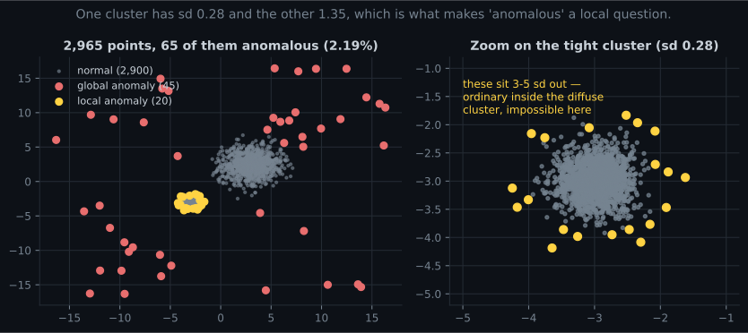
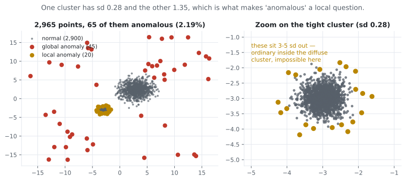
Section titled “Two kinds of anomaly”The data below has 2,965 points and two clusters with deliberately different spreads: one tight (standard deviation 0.28) and one loose (1.35). On top of that sit 65 anomalies of two distinct types.
| Group | Count | What it is |
|---|---|---|
| tight cluster | 1,900 | mean (−3, −3), sd 0.28 |
| loose cluster | 1,000 | mean (3, 2.4), sd 1.35 |
| global anomalies | 45 | uniform, pushed clear of both clusters |
| local anomalies | 20 | ring around the tight cluster at radius 0.9–1.4 |
| anomaly rate | 2.19% |
The distinction is not academic. A transaction of €400 is unremarkable for a business account and extraordinary for a student account; a server at 60% CPU is normal for a database and alarming for a load balancer. Whether a point is anomalous is a question about its neighbourhood, not about the dataset’s global shape — and the two most popular detectors answer different questions.
Six detectors on identical data
Section titled “Six detectors on identical data”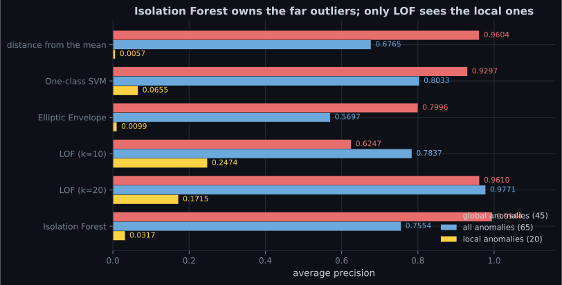
| Detector | All (65) | Global (45) | Local (20) |
|---|---|---|---|
| Isolation Forest | 0.7554 | 0.9944 | 0.0317 |
| LOF (k=20) | 0.9771 | 0.9610 | 0.1715 |
| LOF (k=10) | 0.7837 | 0.6247 | 0.2474 |
| Elliptic Envelope | 0.5697 | 0.7996 | 0.0099 |
| One-class SVM (RBF) | 0.8033 | 0.9297 | 0.0655 |
| distance from the mean | 0.6765 | 0.9604 | 0.0057 |
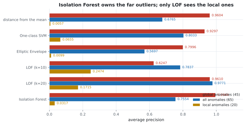
Read the last row first. Euclidean distance from the mean — one line of numpy — reaches 0.9604 on the global anomalies. If your anomalies are of that kind, you do not need a library. What you need a library for is the other kind, and there the same baseline scores 0.0057.
Isolation Forest builds random axis-aligned splits and scores a point by how few splits it takes to isolate. Points in empty regions get isolated fast, which is exactly the global notion — hence 0.9944 and 0.0317. It is also the fastest of the six, has no distance computation, and handles mixed scales without preprocessing.
Local Outlier Factor compares a point’s local density to the density of its neighbours:
where is the inverse of the average reachability distance. The ratio is the point: a LOF of 1 means “as dense as my neighbours”, above 1 means “sparser than my neighbours”. Because it is a ratio, it does not care that the two clusters have different spreads — which is why it is the only method here with any purchase on the local anomalies.
Elliptic Envelope fits one robust Gaussian to everything, so on two clusters it fits an ellipse around both and calls the space between them normal. It is the right tool for genuinely unimodal data and the wrong one here — 0.5697 overall, the worst of the six.
Which detector, and what to do with its output
Section titled “Which detector, and what to do with its output”flowchart TD A["You have unlabelled data
and want the odd rows"] --> B{"Do you have ANY
labelled anomalies,
even 20?"} B -->|"yes"| S["Use them. A supervised model
with class weights beats every
detector here. Keep a detector
only for unseen kinds."] B -->|"no"| C{"What does 'anomalous'
mean for this data?"} C -->|"far from everything --
a sensor reading off by 10x"| G["Distance from the mean,
or Isolation Forest.
Measured 0.96 and 0.99."] C -->|"normal-looking value in the
wrong neighbourhood"| L["LOF. It is the only method
here with any purchase --
and only 0.2474 at best."] C -->|"genuinely unimodal,
one elliptical blob"| E["Elliptic Envelope"] C -->|"unknown or both"| BOTH["Run a global and a local
detector and union the flags.
Report them separately."] G --> P{"How many columns,
and are they all relevant?"} L --> P E --> P BOTH --> P P -->|"irrelevant columns present"| P1["Drop them first.
Distance-based scores drown
in noise dimensions."] P -->|"all relevant"| Q{"How do you pick
contamination?"} P1 --> Q Q -->|"as a model parameter"| Q1["Wrong. It is a budget:
how many rows can a human
review per day?"] Q -->|"as a review budget"| R["Rank by score, review the top n,
and let the labels you collect
turn this into a supervised problem"] Q1 --> R
The loop closing at the bottom is the honest end state. Unsupervised detection is a bootstrap: you use it to generate the labels that let you stop using it. Any project where a detector is still the final answer two years in has usually skipped the step where reviewed flags were written back to a table.
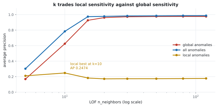
One hyperparameter, no labels
Section titled “One hyperparameter, no labels”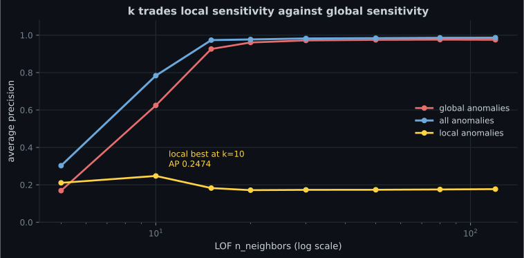
n_neighbors | All | Global | Local |
|---|---|---|---|
| 5 | 0.3025 | 0.1689 | 0.2107 |
| 10 | 0.7837 | 0.6247 | 0.2474 |
| 20 | 0.9771 | 0.9610 | 0.1715 |
| 50 | 0.9841 | 0.9750 | 0.1736 |
| 120 | 0.9864 | 0.9755 | 0.1771 |
The table above is only computable because this page has labels. In production you almost never do — that is what makes anomaly detection different from every other page in this phase. Which means the number you would pick k by does not exist.
What you can do instead:
- Pick k from the domain. If you know an anomaly is a point unlike its 10 nearest peers, that is your k. This is a modelling statement, not a tuning problem.
- Label a sample. A hundred hand-labelled points give a noisy but real AP estimate, and it is far better than nothing. Prioritise labelling the points the detectors disagree about.
- Use synthetic anomalies. Inject known anomalies of the kind you care about, and measure recall on those. It only validates against the anomalies you imagined, which is a real limitation, but it catches gross failures.
- Ensemble across k. Average the scores from several k values, or take the maximum. It gives up peak performance for robustness — a reasonable trade when you cannot measure peak performance anyway.
Irrelevant columns are fatal
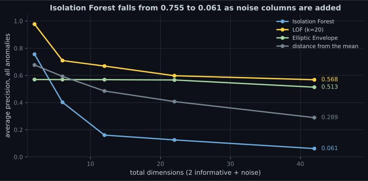
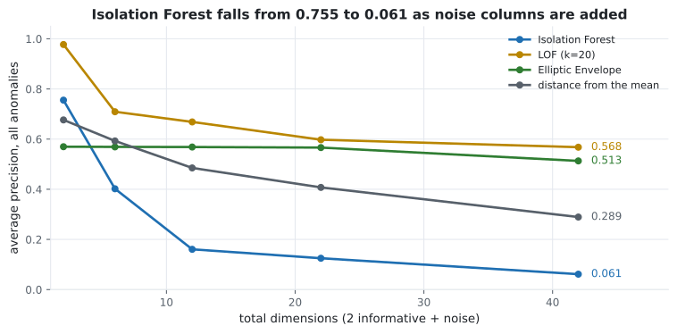
Section titled “Irrelevant columns are fatal”Every real dataset has columns that carry nothing about the anomaly. Here is what they cost:
| Total dimensions | Isolation Forest | LOF (k=20) | Elliptic Envelope | distance from the mean |
|---|---|---|---|---|
| 2 | 0.7554 | 0.9771 | 0.5697 | 0.6765 |
| 6 | 0.4020 | 0.7091 | 0.5690 | 0.5927 |
| 12 | 0.1606 | 0.6685 | 0.5684 | 0.4851 |
| 22 | 0.1250 | 0.5975 | 0.5662 | 0.4074 |
| 42 | 0.0614 | 0.5677 | 0.5130 | 0.2892 |
Three lessons, in decreasing order of how often they are ignored.
Feature selection matters more than model selection here. Going from 42 columns to the 2 that matter improves Isolation Forest by 12× — far more than any switch between detectors. And unlike supervised learning, you have no importance measure to guide you, so this has to come from domain knowledge.
The ranking of methods depends on dimensionality. At 2 dimensions LOF beats Isolation Forest 0.9771 to 0.7554; at 42 it wins 0.5677 to 0.0614. Any blog post declaring one better than the other is describing its own dataset.
Elliptic Envelope’s stability is not a virtue here. It scores 0.5130 at 42 dimensions because it was already only 0.5697 at two: it never fitted the two-cluster structure at all, so there was less to lose.
contamination is not a model parameter
Section titled “contamination is not a model parameter”Every sklearn detector takes contamination, and it is routinely misunderstood as “how sensitive the
model is”. It is not. It converts scores into labels, and nothing else:
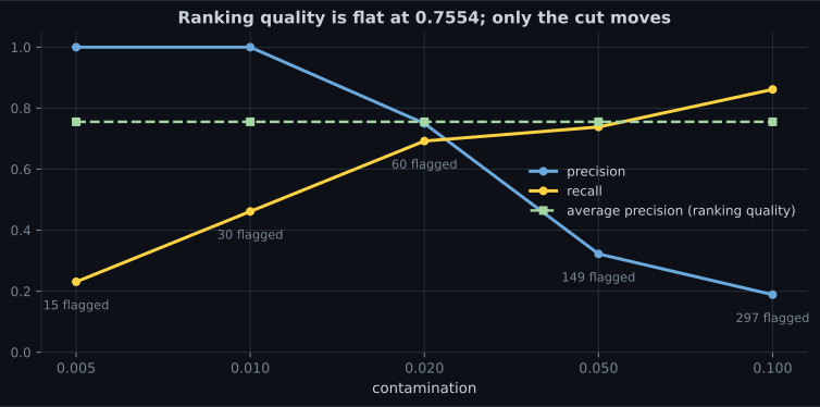
contamination | Flagged | Precision | Recall | Average precision |
|---|---|---|---|---|
| 0.005 | 15 | 1.0000 | 0.2308 | 0.7554 |
| 0.010 | 30 | 1.0000 | 0.4615 | 0.7554 |
| 0.020 | 60 | 0.7500 | 0.6923 | 0.7554 |
| 0.050 | 149 | 0.3221 | 0.7385 | 0.7554 |
| 0.100 | 297 | 0.1886 | 0.8615 | 0.7554 |
This is the threshold discussion
again, in different clothing. contamination is a threshold on the anomaly score, so it trades
precision against recall exactly as any threshold does, and the right value comes from how many alerts
a human can process — not from a grid search.
Two practical consequences:
- Score, then threshold. Use
score_samplesand keep the continuous score. Then flag the top-N per day, where N is your capacity.predict()throws that flexibility away. - Compare models with AP, not with precision. Precision at a fixed contamination conflates ranking quality with the choice of cut, and the numbers above show it can vary by 5× without the model changing at all.
See it move
Section titled “See it move”LOF is a ratio of densities, which is why cluster spread does not fool it. Drag the point and compare what a global distance threshold says with what the local ratio says.
The interesting region is just outside the tight cluster. There, the global criterion says “well within two spreads of the mean, normal” while the local ratio says “far sparser than my neighbours, anomaly”. Inside the loose cluster the disagreement reverses. Every point where the two verdicts differ is a point where your choice of detector decides the answer.
Pitfalls
Section titled “Pitfalls”| Pitfall | Why it bites | What to do |
|---|---|---|
| One detector for all anomaly types | Isolation Forest: 0.9944 global, 0.0317 local | Decide which kind you care about, then choose |
Treating contamination as sensitivity | AP was 0.7554 at every setting | It is the alert budget; score first, threshold second |
Tuning n_neighbors without labels | No k was best for both types | Set it from the domain, or ensemble across k |
| Keeping every column | Isolation Forest 0.7554 → 0.0614 with 40 noise columns | Feature selection beats model selection here |
| Elliptic Envelope on multi-modal data | 0.5697 — worst of six, on two clusters | Only for genuinely unimodal data |
LocalOutlierFactor().predict(X_new) | Raises; novelty=False only supports fit_predict | Set novelty=True when you need to score new points |
| Reporting precision without recall | 1.0000 precision at 15 flagged of 65 anomalies | Report both, plus the alert count |
| Claiming “unsupervised so unmeasurable” | A hundred labels give a usable estimate | Label the disagreements; inject synthetic anomalies |
- 2,965 points, 2.19% anomalous, in two kinds: 45 global and 20 local.
- Isolation Forest: 0.9944 on global anomalies, 0.0317 on local ones. Distance from the mean gets 0.9604 and 0.0057 respectively — global anomalies are easy.
- LOF at k=10 reached 0.2474 on the local anomalies, roughly 8× Isolation Forest, while giving up global performance (0.6247 against 0.9944).
- No k was best at both, and in production there are no labels to choose one with.
- Adding 40 irrelevant columns cost Isolation Forest 12× (0.7554 → 0.0614) and LOF 42%.
contaminationmoved flagged points from 15 to 297 and precision from 1.0000 to 0.1886 while average precision stayed at 0.7554.
-
Isolation Forest gives average precision 0.9944 on your far outliers and 0.0317 on points that are unusual only relative to their neighbours. What is the fix?
Isolation Forest measures how quickly random splits isolate a point, which is a global emptiness criterion. LOF at k=10 reached 0.2474 on exactly those local anomalies — eight times better, and the only method here with any purchase on them.
pch.quizShowAnswer
B — A density-ratio method such as LOF, which compares a point's local density to its neighbours' rather than to the global structure — Isolation Forest measures how quickly random splits isolate a point, which is a global emptiness criterion. LOF at k=10 reached 0.2474 on exactly those local anomalies — eight times better, and the only method here with any purchase on them.
-
You have no labels. How do you choose LOF's n_neighbors?
The measured table shows no k that is best for both anomaly types, so the choice is a modelling statement about which anomalies you care about. A hundred hand-labelled points — ideally the ones detectors disagree about — turn 'no evaluation' into a noisy but real one.
pch.quizShowAnswer
B — From the domain — decide what 'unlike its neighbours' means for your data — or ensemble several k values, and label a sample to sanity-check — The measured table shows no k that is best for both anomaly types, so the choice is a modelling statement about which anomalies you care about. A hundred hand-labelled points — ideally the ones detectors disagree about — turn 'no evaluation' into a noisy but real one.
-
Raising contamination from 0.005 to 0.10 changed precision from 1.0000 to 0.1886 and left average precision at 0.7554. What does that tell you?
The flagged count went from 15 to 297 on identical scores. Keep score_samples output, flag the top N your team can review, and compare models by AP so that ranking quality is not conflated with the choice of cut.
pch.quizShowAnswer
B — contamination only converts scores to labels: the ranking is unchanged, and the parameter is an alert budget rather than a model setting — The flagged count went from 15 to 297 on identical scores. Keep score_samples output, flag the top N your team can review, and compare models by AP so that ranking quality is not conflated with the choice of cut.
-
Adding 40 uninformative columns takes Isolation Forest from 0.7554 to 0.0614. Why is it hit so much harder than Elliptic Envelope?
Elliptic Envelope only looks stable because it started at 0.5697 — it never captured the two-cluster structure, so it had less to lose. The transferable point is that feature selection is worth more here than any choice of detector.
pch.quizShowAnswer
B — Its splits are drawn uniformly over axes, so with 42 columns it spends 95% of its splits on noise; a fitted covariance can down-weight columns that co-vary with nothing — Elliptic Envelope only looks stable because it started at 0.5697 — it never captured the two-cluster structure, so it had less to lose. The transferable point is that feature selection is worth more here than any choice of detector.
-
You call LocalOutlierFactor(n_neighbors=20).fit(X_train).predict(X_new) and get an error. Why?
The two modes answer different questions: outlier detection (which of these points are odd?) against novelty detection (is this new point odd relative to what I have seen?). Set novelty=True for the second, and remember it disables fit_predict.
pch.quizShowAnswer
B — With the default novelty=False, LOF only supports fit_predict on the data it fitted; scoring new points requires novelty=True — The two modes answer different questions: outlier detection (which of these points are odd?) against novelty detection (is this new point odd relative to what I have seen?). Set novelty=True for the second, and remember it disables fit_predict.
🧪 Try It Yourself
Section titled “🧪 Try It Yourself”Exercise 1 – Build both kinds of anomaly
Section titled “Exercise 1 – Build both kinds of anomaly”Exercise 2 – Two detectors, two answers
Section titled “Exercise 2 – Two detectors, two answers”Exercise 3 – Sweep k, and find that no value wins
Section titled “Exercise 3 – Sweep k, and find that no value wins”Exercise 4 – Add columns that contain nothing
Section titled “Exercise 4 – Add columns that contain nothing”Exercise 5 – Show that contamination is only a threshold
Section titled “Exercise 5 – Show that contamination is only a threshold”Phase 10 - Applied ML Problems — the phase overview, with the six measurements from these pages that generalise beyond their own datasets.
pch.coffeeTagline
pch.coffeeCtapch.feedbackHeading
pch.feedbackSubheading