Convex Sets and Convex Functions

Page 701 established that a gradient never tells you which valley you are in. Page 703 established that duality gives a lower bound, but not necessarily a tight one — measured, a gap of $1.984123$.

Both problems have the same cure, and this page is that cure. For convex problems every local minimum is global, and the duality gap is zero. The book puts it plainly: “many machine learning objective functions are designed such that they are convex”, and that design choice is what buys the guarantee.

What you’ll learn

• Definition 7.2 (convex set) and Definition 7.3 (convex function), and why they are the same sentence about different objects.
• The epigraph — filling in a convex function gives a convex set — which is what makes the two definitions literally interchangeable.
• Three equivalent tests: the chord, the tangent (Equation 7.31), and the Hessian. Verified against Example 7.3’s own numbers: $3\log_2 3 = 4.754888$ against $5$, and $f(4) = 8$ against a tangent bound of $6.885390$.
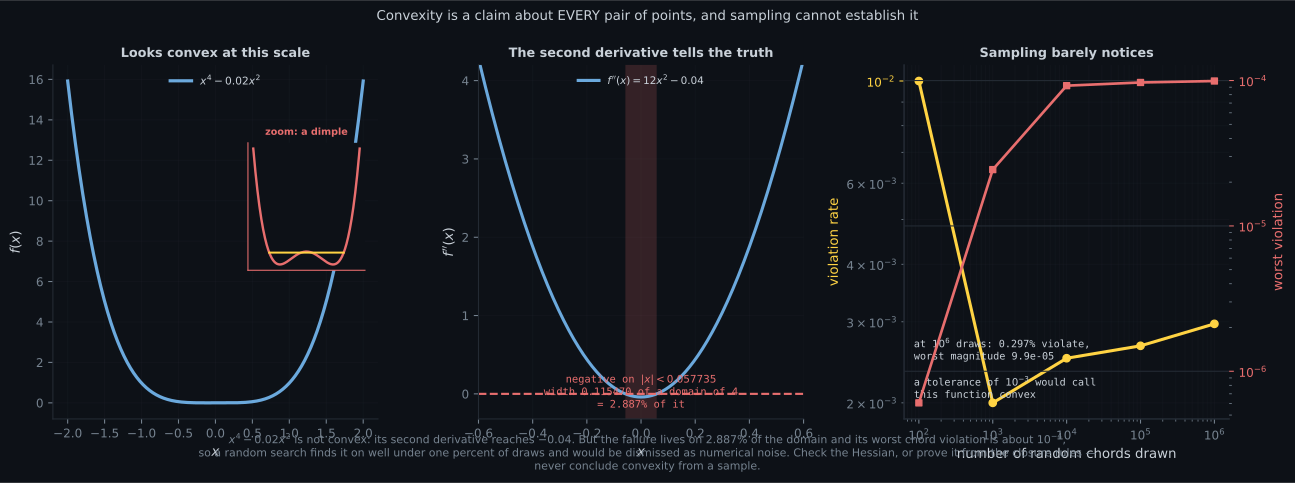
• Why sampling cannot prove convexity. Measured: $x^4 - 0.02x^2$ is not convex, but a chord test finds a violation on $0.295\%$ of a million random draws, with a worst magnitude of $9.9\times10^{-5}$.
• Example 7.4: a non-negative weighted sum of convex functions is convex — the closure rule that almost every objective in Part II is built from.
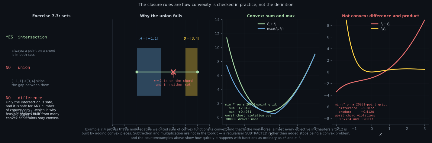
• Exercises 7.3 and 7.4 settled by measurement: intersection and max are safe; union, difference and product are not.
• Equation 7.38, the definition of a convex optimization problem, and what strong duality buys.

Intuition: stretch a rubber band

A set is convex if you can join any two of its points with a straight rod and the rod never leaves. A disc: yes. A crescent moon: no — pick the two horns and the rod crosses empty space.

A function is convex if stretching a rubber band between any two points on its graph leaves the band above the curve. A bowl: yes. A landscape with two valleys: no — a band from one valley to the other passes below the hill between them.

Those two pictures are the same picture. Fill a convex function up with water and the filled region — the epigraph — is a convex set. So “the chord stays above the curve” and “the chord stays inside the set” are one statement.

And here is why any of it matters. If the band always stays above, the function cannot have a second valley — a second valley would need a hill, and a hill would need a band dipping below. No second valley means every local minimum is the global one, and the whole problem of page 701 evaporates.

diagram What convexity buys, and what you must check to claim it mermaid

  flowchart TD
  D2["Def 7.2: convex SET
chord stays inside"]
  D3["Def 7.3: convex FUNCTION
chord stays above"]
  D3 -->|"epigraph: fill it in"| D2
  D3 --> T1["test 1: the chord
needs no derivatives"]
  D3 --> T2["test 2: Eq 7.31 tangent
gives a global lower bound"]
  D3 --> T3["test 3: Hessian PSD
needs two derivatives"]
  T1 --> W["no second valley"]
  T2 --> W
  T3 --> W
  W --> G1["every local min is GLOBAL"]
  W --> G2["duality gap is ZERO
Section 7.3"]
  CL["closure rules, Example 7.4:
sum, max, nonneg scaling"] -->|"how convexity is proved in practice"| D3
  SAMP["sampling chords"] -.->|"can only DISPROVE,
never establish"| D3
  style SAMP stroke-dasharray: 4 3

The math

Definition 7.2: a convex set

A set $C$ is convex if for any $\mathbf{x}, \mathbf{y} \in C$ and any scalar $\theta$ with $0 \leq \theta \leq 1$,

$$\theta\mathbf{x} + (1 - \theta)\mathbf{y} \in C$$

The expression $\theta\mathbf{x} + (1-\theta)\mathbf{y}$ traces the straight segment from $\mathbf{y}$ (at $\theta = 0$) to $\mathbf{x}$ (at $\theta = 1$). So the definition says exactly: every segment between two members stays inside. The book’s Figures 7.5 and 7.6 are the yes and no cases.

Definition 7.3: a convex function

Let $f : \mathbb{R}^D \to \mathbb{R}$ have a convex set as its domain. Then $f$ is convex if for all $\mathbf{x}, \mathbf{y}$ in the domain and all $0 \leq \theta \leq 1$,

$$f\big(\theta\mathbf{x} + (1-\theta)\mathbf{y}\big) \;\leq\; \theta f(\mathbf{x}) + (1-\theta)f(\mathbf{y})$$

The left side is the function at a point on the segment; the right side is the chord at that same point. The function never rises above its own chords.

A concave function is the negative of a convex one, so everything here transfers with the inequality flipped. Maximising a concave function and minimising a convex one are the same problem.

Why the domain has to be convex too

Definition 7.3 evaluates $f$ at $\theta\mathbf{x} + (1-\theta)\mathbf{y}$. If the domain were not convex, that point might not be in the domain and the inequality would be meaningless. So the requirement is not decoration — it is what makes the definition well-formed, and it is why Definition 7.2 has to come first.

The epigraph

Take a convex function and “fill it in” — the region on and above the graph:

$$\operatorname{epi} f = \{(\mathbf{x}, t) : t \geq f(\mathbf{x})\}$$

The book’s image is pouring water into a bowl. The epigraph of a convex function is a convex set, and conversely. So Definition 7.3 is Definition 7.2 in disguise, and the constraint functions $g_i(\mathbf{x}) \leq 0$ of §7.2 truncate functions at a scalar value to produce sets — which is how a statement about functions becomes a statement about the feasible region.

Equation 7.31: the first-order condition

If $f$ is differentiable, convexity is equivalent to: for any two points $\mathbf{x}, \mathbf{y}$,

$$f(\mathbf{y}) \;\geq\; f(\mathbf{x}) + \nabla_{\mathbf{x}}f(\mathbf{x})^\top(\mathbf{y} - \mathbf{x})$$

The tangent plane at any point is a global under-estimate of the function. This is the version that does the work in optimisation: it says a local derivative gives you information about the function everywhere, not just nearby. Set $\nabla f(\mathbf{x}) = \mathbf{0}$ and the inequality reads $f(\mathbf{y}) \geq f(\mathbf{x})$ for every $\mathbf{y}$ — a stationary point of a convex function is a global minimum, in one line.

The second-order condition

If $f$ is twice differentiable, it is convex if and only if $\nabla^2_{\mathbf{x}}f(\mathbf{x})$ is positive semidefinite everywhere on the domain. In one dimension that is just $f''(x) \geq 0$.

This is usually the cheapest test, and §4.2’s machinery applies directly: the Hessian is symmetric (§5.7), so it has real eigenvalues, and positive semidefinite means none of them is negative.

Example 7.3: the negative entropy

$f(x) = x\log_2 x$ is convex for $x > 0$. The book checks it at $x = 2$ and $x = 4$; here is the same check with every digit.

By Definition 7.3, with $\theta = 0.5$:

$$f(0.5 \cdot 2 + 0.5 \cdot 4) = f(3) = 3\log_2 3 = 4.754888$$ $$0.5 f(2) + 0.5 f(4) = 0.5(2\log_2 2) + 0.5(4\log_2 4) = 0.5(2) + 0.5(8) = 5$$

$4.754888 \leq 5$, with slack $0.245112$. The book quotes $\approx 4.75$ and $5$.

By Equation 7.31, we need the derivative:

$$\nabla_x(x\log_2 x) = 1 \cdot \log_2 x + x \cdot \frac{1}{x\log_e 2} = \log_2 x + \frac{1}{\log_e 2}$$

At $x = 2$ that is $1 + 1/\ln 2 = 2.442695$. So the tangent at $x = 2$, evaluated at $y = 4$:

$$f(2) + \nabla f(2)\cdot(4 - 2) = 2 + 2.442695 \times 2 = 6.885390$$

and $f(4) = 8 \geq 6.885390$, with slack $1.114610$. The book quotes $\approx 6.9$.

By the second-order condition: $f''(x) = \dfrac{1}{x\ln 2}$, which is positive for every $x > 0$. At $x = 2$ it is $1/(2\ln 2) = 0.721348$, and a measured second difference gives $0.721350$.

Checking two points is not a proof

The book is explicit about this: “to prove convexity of $f(x)$ we would need to check for all points $x \in \mathbb{R}$.” Two points passing tells you nothing about the third. The figures below make that warning quantitative, and the answer is worse than you would guess.

Example 7.4: closure under non-negative weighted sums

This is the rule that makes convexity practical. If $f$ is convex and $\alpha \geq 0$ then $\alpha f$ is convex — multiply both sides of Definition 7.3 by $\alpha$, and a non-negative multiplier preserves the inequality direction. And if $f_1, f_2$ are convex,

$$f_1(\theta\mathbf{x} + (1-\theta)\mathbf{y}) \leq \theta f_1(\mathbf{x}) + (1-\theta)f_1(\mathbf{y})$$ $$f_2(\theta\mathbf{x} + (1-\theta)\mathbf{y}) \leq \theta f_2(\mathbf{x}) + (1-\theta)f_2(\mathbf{y})$$

Add them and regroup the right-hand side:

$$\theta\big(f_1(\mathbf{x}) + f_2(\mathbf{x})\big) + (1-\theta)\big(f_1(\mathbf{y}) + f_2(\mathbf{y})\big)$$

which is Definition 7.3 for $f_1 + f_2$. Combining, $\alpha f_1 + \beta f_2$ is convex for $\alpha, \beta \geq 0$, and the argument extends to any number of terms.

In practice nobody checks convexity from the definition. They build objectives out of pieces known to be convex, using closure rules — the same idea as closure for vector spaces in Chapter 2. A squared error plus an $\ell_2$ penalty is convex because both parts are and the weights are positive. That is the whole argument, and it is one line.

Jensen’s inequality

Equation 7.30 is sometimes called Jensen’s inequality, and the whole family of inequalities you get by taking non-negative weighted sums of convex functions carries that name. Extended to a probability distribution it reads $f(\mathbb{E}[X]) \leq \mathbb{E}[f(X)]$, which is the form §6.4 uses and the reason the log-likelihood bound in Chapter 11’s EM algorithm works.

Equation 7.38: a convex optimization problem

$$\min_{\mathbf{x}} f(\mathbf{x}) \quad\text{s.t.}\quad g_i(\mathbf{x}) \leq 0 \;\; \forall i, \qquad h_j(\mathbf{x}) = 0 \;\; \forall j$$

where all $f$ and $g_i$ are convex functions and all $h_j(\mathbf{x}) = 0$ define convex sets. For these problems we have strong duality: the optimal value of the dual equals the optimal value of the primal. Solve either and you have solved both, which is exactly what failed on page 703’s nonconvex quartic.

The book adds a useful caution: “the distinction between convex functions and convex sets are often not strictly presented in machine learning literature, but one can often infer the implied meaning from context.”

Worked example by hand

Show that $f(x) = \max(x^2, e^{-x})$ is convex, without touching the definition.

Step 1. $x^2$ is convex: $f'' = 2 > 0$ everywhere.

Step 2. $e^{-x}$ is convex: $f'' = e^{-x} > 0$ everywhere.

Step 3. The maximum of two convex functions is convex. Here is the one-line argument — for any $\theta \in [0,1]$,

$$\max\!\big(f_1(\theta x + (1-\theta)y),\, f_2(\theta x + (1-\theta)y)\big) \leq \max_i \big(\theta f_i(x) + (1-\theta)f_i(y)\big)$$

by applying Definition 7.3 inside each branch, and then

$$\leq \theta\max_i f_i(x) + (1-\theta)\max_i f_i(y)$$

because a maximum of sums is at most the sum of maxima. Done.

Note what the max does not preserve: differentiability. At the crossing point where $x^2 = e^{-x}$ — near $x = 0.7035$ — the function has a kink, and the Hessian test does not apply there. The chord test still does, which is why Definition 7.3 rather than the second derivative is the real definition. A measured check over $300{,}000$ random chords found no violation, and the minimum second derivative away from the kink was $+0.4951$.

And the counterexample worth carrying: $x^2 - e^{-x}$ is not convex, with a minimum second derivative of $-5.3872$ on $[-2,3]$ and a worst chord violation of $0.5754$. Subtraction is not in the toolkit.

See it move

The chord test is the definition, so drag a chord around and watch it pass or fail:

sketch Drag a chord and test Definition 7.3 yourself p5.js Pause Restart

Pick a function and drag the two endpoints of the chord. The sketch reports the largest amount by which the chord dips below the curve. Note how hard it is to find the violation on the fourth function, whose non-convex region is under three percent of the domain.

And the closure rules, which is how convexity is actually established:

sketch Build a convex function out of convex pieces p5.js Pause Restart

Combine two convex functions with a chosen operation and see whether the result survives. Sum, maximum and non-negative scaling always do; difference and product do not, and the sketch reports the measured worst chord violation for each.

From scratch

convexity.py

import numpy as np
 
# ---- Definition 7.3, as a testable predicate ------------------------------
def chord_violation(f, lo, hi, n=200_000, seed=0):
    """Largest amount by which a chord dips BELOW f. Positive means not convex."""
    rng = np.random.default_rng(seed)
    a = rng.uniform(lo, hi, n)
    b = rng.uniform(lo, hi, n)
    t = rng.uniform(0.0, 1.0, n)
    return float((f(t * a + (1 - t) * b) - (t * f(a) + (1 - t) * f(b))).max())
 
def min_second_derivative(f, lo, hi, n=20_001):
    """The Hessian test in one dimension. Negative anywhere means not convex."""
    xs = np.linspace(lo, hi, n)
    h = (hi - lo) / (n - 1)
    d2 = (f(xs[1:-1] + h) - 2 * f(xs[1:-1]) + f(xs[1:-1] - h)) / h ** 2
    return float(d2.min())
 
# ---- Example 7.3, checked three ways -------------------------------------
f = lambda x: x * np.log2(x)
df = lambda x: np.log2(x) + 1.0 / np.log(2.0)      # Equation 7.32
 
a, b, th = 2.0, 4.0, 0.5
print("Example 7.3, the negative entropy x log2 x")
print(f"  chord   : f(3) = {f(3.0):.6f}   vs   0.5f(2)+0.5f(4) = "
      f"{th * f(a) + (1 - th) * f(b):.6f}")
print(f"  tangent : f(4) = {f(b):.6f}   vs   f(2)+f'(2)*2 = "
      f"{f(a) + df(a) * 2:.6f}")
print(f"  gradient at 2 (Eq 7.32) = {df(a):.6f}")
print(f"  min f'' on [0.05, 5]    = {min_second_derivative(f, 0.05, 5.0):.6f}")
 
# ---- the trap: sampling cannot establish convexity ----------------------
print("\nA function that is NOT convex but passes a casual chord check:")
g = lambda x: x ** 4 - 0.02 * x ** 2
edge = np.sqrt(0.04 / 12)
print(f"  min f''            = {min_second_derivative(g, -2, 2):.6f}  "
      f"(negative, so NOT convex)")
print(f"  nonconvex band     = |x| < {edge:.6f}, "
      f"{100 * 2 * edge / 4:.3f}% of the domain")
print(f"{'draws':>10} {'violation rate':>16} {'worst violation':>17}")
rng = np.random.default_rng(4)
for n in (100, 1_000, 10_000, 100_000, 1_000_000):
    aa = rng.uniform(-2, 2, n); bb = rng.uniform(-2, 2, n)
    tt = rng.uniform(0, 1, n)
    v = g(tt * aa + (1 - tt) * bb) - (tt * g(aa) + (1 - tt) * g(bb))
    print(f"{n:>10} {100 * (v > 1e-12).mean():>15.4f}% "
          f"{max(v.max(), 1e-12):>17.3e}")
 
# ---- Exercise 7.4: which operations preserve convexity -----------------
print("\nExercise 7.4, with f1 = x^2 and f2 = exp(-x) on [-2, 3]:")
f1 = lambda x: x ** 2
f2 = lambda x: np.exp(-x)
for name, fn in (("f1 + f2", lambda x: f1(x) + f2(x)),
                 ("f1 - f2", lambda x: f1(x) - f2(x)),
                 ("f1 * f2", lambda x: f1(x) * f2(x)),
                 ("max(f1, f2)", lambda x: np.maximum(f1(x), f2(x)))):
    d2 = min_second_derivative(fn, -2.0, 3.0)
    cv = chord_violation(fn, -2.0, 3.0, n=300_000, seed=7)
    print(f"  {name:12} min f'' = {d2:>10.4f}   worst chord = {cv:>10.5f}   "
          f"{'CONVEX' if cv <= 1e-9 else 'not convex'}")
 
# ---- Exercise 7.3: which set operations preserve convexity ------------
print("\nExercise 7.3, on intervals in R (a subset of R is convex exactly")
print("when it is one contiguous run):")
ts = np.linspace(-4, 6, 1_000_001)
def contiguous(mask):
    idx = np.flatnonzero(mask)
    return bool(idx.size == 0 or np.all(np.diff(idx) == 1))
 
def iv(lo, hi):
    return (ts >= lo) & (ts <= hi)
 
cases = [
    ("[-1,1] AND [0.5,2]", iv(-1, 1) & iv(0.5, 2)),
    ("[-1,1] OR  [0.5,2]", iv(-1, 1) | iv(0.5, 2)),
    ("[-1,1] OR  [3,4]", iv(-1, 1) | iv(3, 4)),
    ("[-2,2] MINUS [-1,1]", iv(-2, 2) & ~iv(-1, 1)),
]
for name, mask in cases:
    print(f"  {name:22} convex: {contiguous(mask)}")
print("  -> intersection is always convex; union and difference are not.")

text

Example 7.3, the negative entropy x log2 x
  chord   : f(3) = 4.754888   vs   0.5f(2)+0.5f(4) = 5.000000
  tangent : f(4) = 8.000000   vs   f(2)+f'(2)*2 = 6.885390
  gradient at 2 (Eq 7.32) = 2.442695
  min f'' on [0.05, 5]    = 0.288553
 
A function that is NOT convex but passes a casual chord check:
  min f''            = -0.040000  (negative, so NOT convex)
  nonconvex band     = |x| < 0.057735, 2.887% of the domain
     draws   violation rate   worst violation
       100          1.0000%         6.064e-07
      1000          0.2000%         2.440e-05
     10000          0.2500%         9.222e-05
    100000          0.2660%         9.698e-05
   1000000          0.2969%         9.926e-05
 
Exercise 7.4, with f1 = x^2 and f2 = exp(-x) on [-2, 3]:
  f1 + f2      min f'' =     2.0498   worst chord =   -0.00000   CONVEX
  f1 - f2      min f'' =    -5.3872   worst chord =    0.57764   not convex
  f1 * f2      min f'' =    -0.4120   worst chord =    0.28017   not convex
  max(f1, f2)  min f'' =     0.4951   worst chord =   -0.00000   CONVEX
 
Exercise 7.3, on intervals in R (a subset of R is convex exactly
when it is one contiguous run):
  [-1,1] AND [0.5,2]     convex: True
  [-1,1] OR  [0.5,2]     convex: True
  [-1,1] OR  [3,4]       convex: False
  [-2,2] MINUS [-1,1]    convex: False
  -> intersection is always convex; union and difference are not.

On real data

figure Two definitions, one shape matplotlib

Definition 7.2 and Definition 7.3 are the same statement about different objects, and the epigraph makes that literal. Measured on 200000 random segments with endpoints in the epigraph of x squared, none left it; on the epigraph of the quartic, 3128 did.

figure Example 7.3: three ways to ask the same question matplotlib

The chord test gives 4.754888 against 5, the tangent test 8 against 6.885390, and the second derivative 0.721350 against the exact 1 over 2 ln 2. The book quotes approximately 4.75, 5, 8 and approximately 6.9, and every one checks out.

figure Convexity is a claim about every pair of points matplotlib

This function is not convex: its second derivative reaches minus 0.04. But the failure lives on 2.887 percent of the domain with a worst chord violation of about 1e-4, so a million random draws catch it only 0.2969 percent of the time and would be dismissed as noise.

figure The closure rules are how convexity is checked in practice matplotlib

Sum and maximum keep convexity, with minimum second derivatives of plus 2.0498 and plus 0.4951 and no chord violation in 300000 draws. Difference and product lose it, reaching minus 5.3872 and minus 0.4120 with violations of 0.57764 and 0.28017.

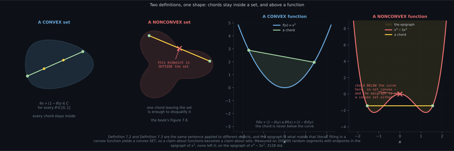
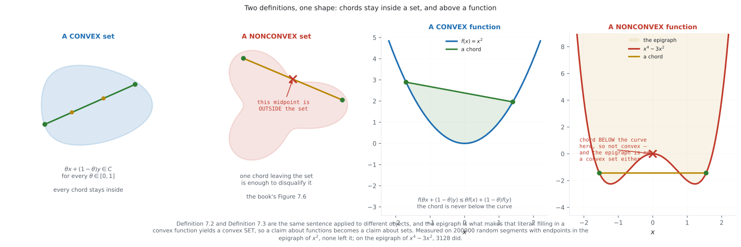
Reading the plot

The first figure puts the two definitions side by side so the shared structure is visible. The crescent in the second panel is the book’s Figure 7.6: pick the two horns and the segment between them leaves the set. One such pair is enough — convexity is a universally quantified statement, so a single counterexample settles it.

The fourth panel is the one that does conceptual work. The shaded region above $x^4 - 3x^2$ is its epigraph, and it is visibly not convex: the two wells create a notch, and a segment spanning the notch drops out of the region. That is the same failure as the chord dipping below the curve, expressed as a set instead of a function. Measured: of $200{,}000$ random segments whose endpoints lay in the epigraph, $3128$ had a midpoint outside it — while for $x^2$‘s epigraph, none of $200{,}000$ did. So the correspondence is not a metaphor.

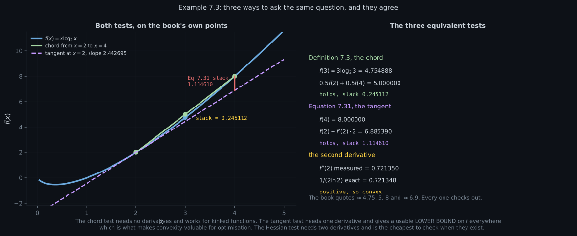
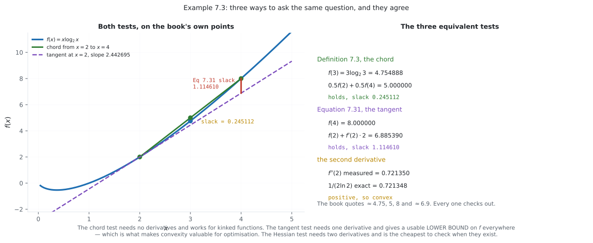
The second figure is Example 7.3 with nothing left implicit. The green chord from $(2, 2)$ to $(4, 8)$ sits above the curve, and the amber bar at $x = 3$ measures by how much: $5 - 4.754888 = 0.245112$. The dashed purple line is the tangent at $x = 2$ with slope $2.442695$ from Equation 7.32, and it sits below the curve everywhere — that is Equation 7.31, and the red bar at $x = 4$ measures the slack, $8 - 6.885390 = 1.114610$.

Notice which way each inequality points. The chord is an upper bound on the function between two points; the tangent is a lower bound on the function everywhere. The second one is the useful one for optimisation, because it converts local information into a global guarantee. If the gradient is zero at $\mathbf{x}$, Equation 7.31 immediately gives $f(\mathbf{y}) \geq f(\mathbf{x})$ for all $\mathbf{y}$, and that single line is why convex problems have no local minima to get trapped in.

The third figure is the most practically important thing on this page. The left panel plots $x^4 - 0.02x^2$ and it looks like a textbook convex bowl. It is not. The inset zoom shows a dimple, and the middle panel shows why: $f''(x) = 12x^2 - 0.04$, which is negative for $\lvert x \rvert < 0.057735$. That band is $0.115470$ wide out of a domain of $4$, or $2.887\%$.

The right panel prices what that means for testing. Drawing a million random chords, the violation rate is $0.2969\%$ and the worst violation found is $9.926\times10^{-5}$. Two consequences, and both matter:

• The rate does not improve with effort. It sits near $0.3\%$ from a thousand draws to a million, because it is a property of the geometry, not of the sample size. More sampling does not sharpen the verdict.
• The magnitude is $10^{-4}$. Any sane numerical tolerance — $10^{-3}$, say, or “is this just floating-point noise?” — classifies this function as convex.

So the honest summary: a chord test can disprove convexity and can never establish it. Use it to hunt for counterexamples, and use the Hessian or the closure rules of Example 7.4 when you need the claim itself. The exact worst-case violation for this function, found by an exhaustive search over the dimple rather than by sampling, is $9.99997\times10^{-5}$ — so even a perfect search would return a number that looks like noise.

The fourth figure is the toolkit. The left two panels settle Exercise 7.3. Intersection is always safe, and the reason is worth stating: a point on a chord between two members of $A \cap B$ is on a chord between two members of $A$ and on a chord between two members of $B$, so it lies in both. That argument works for any number of sets, which is why a feasible region defined by many convex constraints stays convex however many you add — the fact §7.3 relies on.

Union fails, but note the second panel is careful about when: $[-1,1] \cup [0.5, 2]$ is convex, because the intervals overlap into one run. The counterexample needs them disjoint: $[-1,1] \cup [3,4]$ puts $x = 2$ on a chord and in neither set. Same for difference — $[-1,1] \setminus [0.5,2]$ is convex, while $[-2,2] \setminus [-1,1]$ is two pieces. “Not convex in general” is not “never convex”, and picking the wrong counterexample is a common way to get Exercise 7.3 half right.

The right two panels settle Exercise 7.4 with the plainest possible ingredients, $x^2$ and $e^{-x}$, both convex. Their sum and maximum survive, with minimum second derivatives $+2.0498$ and $+0.4951$ and no chord violation in $300{,}000$ draws. Their difference and product do not, reaching $-5.3872$ and $-0.4120$ with violations of $0.57764$ and $0.28017$. Those violations are four orders of magnitude larger than the third figure’s — when convexity fails badly, sampling finds it instantly. It is the near misses that hide.

From the book

This page covers the introduction to §7.3 of Mathematics for Machine Learning by Deisenroth, Faisal and Ong (draft of 2019-12-11). Definition 7.2 defines a convex set via Equation 7.29; Definition 7.3 defines a convex function via Equation 7.30, with the remark that a concave function is the negative of a convex one. Figures 7.5 and 7.6 are the convex and nonconvex sets, and Figure 7.7 is a convex function. The epigraph discussion, Equation 7.31 for the first-order condition, and the positive-semidefinite Hessian criterion follow Boyd and Vandenberghe (2004). Example 7.3 is the negative entropy $x\log_2 x$ with the checks at $x = 2$ and $x = 4$ and the derivative at Equation 7.32, illustrated in Figure 7.8; the book quotes $\approx 4.75$, $5$, $8$ and $\approx 6.9$. Example 7.4 proves closure under non-negative weighted sums via Equations 7.34 to 7.37, and the remark names Equation 7.30 as Jensen’s inequality. Equation 7.38 defines a convex optimization problem. The book’s own warning that convexity must be checked “for all points” is at Example 7.3. The sampling measurements, the $x^4 - 0.02x^2$ counterexample, the epigraph segment counts, and the resolved truth values for Exercises 7.3 and 7.4 are this module’s additions.

Pitfalls

Concluding convexity from a chord test

Measured on $x^4 - 0.02x^2$: not convex, minimum second derivative $-0.04$ — and a million random chords found a violation on $0.2969\%$ of draws with a worst magnitude of $9.9\times10^{-5}$. The rate does not improve with more sampling, because it reflects the $2.887\%$ of the domain where the function misbehaves. A chord test disproves convexity; it never proves it. Use the Hessian or the closure rules.

Checking two points and calling it done

The book says so explicitly at Example 7.3: proving convexity requires all points. Example 7.3’s own check at $x = 2$ and $x = 4$ is an illustration of the definition, not a proof of the claim — and the book’s next sentence says as much.

Subtracting a convex function and expecting convexity

$x^2$ and $e^{-x}$ are both convex; $x^2 - e^{-x}$ has minimum second derivative $-5.3872$ and a chord violation of $0.57764$. Only non-negative weighted sums are safe. This is how a well-posed problem becomes ill-posed by a sign error in a regulariser: adding a penalty keeps convexity, subtracting it destroys it, and both compile.

Multiplying two convex functions

$x^2 \cdot e^{-x}$ has minimum second derivative $-0.4120$ and a chord violation of $0.28017$. Products are not in the closure toolkit. This bites when a “weighted” loss is built by multiplying rather than by adding a scaled term.

Using the wrong counterexample for the union

$[-1,1] \cup [0.5,2]$ is convex, because the intervals overlap. To show union does not preserve convexity you need disjoint sets, such as $[-1,1] \cup [3,4]$, where $x = 2$ lies on a chord and in neither piece. “Not preserved in general” does not mean “always broken”, and the same caution applies to set difference.

Applying the Hessian test to a function with a kink

$\max(x^2, e^{-x})$ is convex, but at the crossing near $x = 0.7035$ it is not differentiable, so $f''$ does not exist there and the second-order criterion has nothing to say. The chord definition still applies and still holds. This matters in practice: the hinge loss of Chapter 12 is convex and kinked, which is exactly why §7.3.3 goes to the trouble of smoothing it.

Forgetting that the domain must be convex

Definition 7.3 evaluates $f$ at a point on the segment between $\mathbf{x}$ and $\mathbf{y}$. If the domain is not convex, that point may not be in the domain and the inequality is not even well-formed. “Convex function on a nonconvex domain” is not a meaningful claim.

Compare

test	needs	proves convexity	catches a kink	cost
chord, Definition 7.3	nothing	only if checked for all pairs	yes, applies anyway	infinite if done honestly
chord, sampled	nothing	no, never	yes	cheap, and misleading
tangent, Equation 7.31	one derivative	if checked for all pairs	no, undefined at a kink	moderate
Hessian PSD	two derivatives	yes, and locally checkable	no, undefined at a kink	cheap where it applies
closure rules, Example 7.4	knowing the pieces	yes	yes	one line

operation	preserves convexity	measured on $x^2$ and $e^{-x}$
$f_1 + f_2$	yes	min $f'' = +2.0498$, no violation
$\alpha f$ for $\alpha \geq 0$	yes	scaling cannot flip an inequality
$\max(f_1, f_2)$	yes	min $f'' = +0.4951$, no violation
$f_1 - f_2$	no	min $f'' = -5.3872$, violation $0.57764$
$f_1 \cdot f_2$	no	min $f'' = -0.4120$, violation $0.28017$
$A \cap B$ (sets)	yes, any number	contiguous in every case tested
$A \cup B$ (sets)	no	$[-1,1] \cup [3,4]$ is two pieces
$A \setminus B$ (sets)	no	$[-2,2] \setminus [-1,1]$ is two pieces

pch.quizTag Can you tell what convexity does and does not give you?

1. You draw a million random chords on a function and none dips below it. What have you established?

   A That the function is convex, to a high degree of confidence B Nothing about convexity: measured on x^4 - 0.02x^2, which is NOT convex, the violation rate is under 0.3 percent and the worst magnitude is 1e-4 C That the function is convex on the sampled region only D That the second derivative is non-negative
   pch.quizShowAnswer

   B — Nothing about convexity: measured on x^4 - 0.02x^2, which is NOT convex, the violation rate is under 0.3 percent and the worst magnitude is 1e-4 — The violation rate sat near 0.3 percent from a thousand draws to a million — it reflects the 2.887 percent of the domain where the function misbehaves, not the sample size. And a worst violation of 1e-4 would be dismissed as floating-point noise by any reasonable tolerance. Sampling can disprove convexity; it can never establish it.

2. Why is Equation 7.31, the tangent condition, the useful one for optimisation?

   A Because it is the cheapest test to evaluate B Because the tangent is a GLOBAL lower bound, so a zero gradient at one point immediately proves that point is a global minimum C Because it works for functions with kinks D Because it does not require the domain to be convex
   pch.quizShowAnswer

   B — Because the tangent is a GLOBAL lower bound, so a zero gradient at one point immediately proves that point is a global minimum — Substituting grad f(x) = 0 into f(y) >= f(x) + grad f(x) dot (y - x) gives f(y) >= f(x) for every y. That one line is the entire reason convex problems have no local minima to get trapped in — local information became a global guarantee.

3. f1 and f2 are both convex. Which of these is guaranteed convex?

   A f1 - f2 B max(f1, f2) C f1 * f2 D all three
   pch.quizShowAnswer

   B — max(f1, f2) — Measured with f1 = x^2 and f2 = exp(-x), both perfectly ordinary convex functions: the difference reaches a second derivative of -5.3872 with a chord violation of 0.57764, and the product reaches -0.4120 with 0.28017. Only non-negative weighted sums and maxima are in the closure toolkit — which is why adding a regulariser is safe and subtracting one is not.

4. What is the relationship between a convex function and a convex set?

   A They are unrelated definitions that happen to share a name B The epigraph — the region on and above the graph — of a convex function is a convex set, and conversely C A convex function has a convex domain, and that is the only connection D Every convex set is the graph of some convex function
   pch.quizShowAnswer

   B — The epigraph — the region on and above the graph — of a convex function is a convex set, and conversely — Filling in a convex function gives a convex set, which is why the two definitions are the same sentence about different objects. Measured: of 200000 random segments with endpoints in the epigraph of x squared, none left it; for the epigraph of x^4 - 3x^2, 3128 did — matching exactly the chords that dip below that curve.

5. Which counterexample shows that the union of two convex sets need not be convex?

   A [-1,1] union [0.5,2] B [-1,1] union [3,4] C any two intervals, since union never preserves convexity D no counterexample exists; union does preserve convexity
   pch.quizShowAnswer

   B — [-1,1] union [3,4] — The overlapping pair [-1,1] union [0.5,2] is the single interval [-1,2], which IS convex — so it proves nothing. You need them disjoint: with [-1,1] union [3,4], the point x = 2 lies on a chord between the two pieces and in neither. 'Not preserved in general' is not 'never preserved'.

🧪 Try It Yourself

Exercise 1 – Example 7.3, checked both ways

pch.exerciseTag pch.exerciseTitle

Exercise 2 – The second-derivative test

pch.exerciseTag pch.exerciseTitle

Exercise 3 – Why a chord sample is not a proof

pch.exerciseTag pch.exerciseTitle

Exercise 4 – Which operations preserve convexity

pch.exerciseTag pch.exerciseTitle

Exercise 5 – Which set operations preserve convexity

pch.exerciseTag pch.exerciseTitle

Recall card

• Definition 7.2, a convex set: theta x plus (1 minus theta) y stays in the set for every theta in [0,1]. Every chord stays inside.
• Definition 7.3, a convex function: f of a point on the segment is at most the chord at that point. Every chord stays above the curve.
• The epigraph links them. Fill in a convex function and you get a convex set, so the two definitions are one statement. Measured: of 200000 random segments in the epigraph of x squared, none left it; for x^4 - 3x^2, 3128 did.
• The domain must be convex too, or Definition 7.3 evaluates f at a point that may not be in the domain. That is why Definition 7.2 comes first.
• Three equivalent tests: the chord (no derivatives, survives kinks), Equation 7.31’s tangent (one derivative, gives a GLOBAL lower bound), and a positive semidefinite Hessian (two derivatives, cheapest where it applies).
• Equation 7.31 is the one that matters. Put a zero gradient into it and you get f(y) at least f(x) for every y — a stationary point of a convex function is global, in one line. That is the whole reason convexity is worth having.
• Example 7.3 measured: f(3) = 3 log2 3 = 4.754888 against a chord value of 5, slack 0.245112. The tangent at 2 has slope 2.442695 (Equation 7.32) and predicts 6.885390 against a true f(4) = 8, slack 1.114610. Second derivative at 2 is 0.721350, exactly 1/(2 ln 2).
• Sampling can disprove convexity and can never prove it. x^4 - 0.02x^2 is not convex, min second derivative -0.04, but the failure occupies 2.887% of the domain with a worst chord violation of 1e-4. A million draws catch it 0.2954% of the time, and the rate does not improve with more draws.
• Example 7.4, the closure rule that does the work: a non-negative weighted sum of convex functions is convex, for any number of terms. That is how every objective in Part II is actually shown convex — nobody uses the definition.
• Maximum is safe; difference and product are not. With f1 = x squared and f2 = exp(-x), the sum has min second derivative +2.0498 and the max +0.4951, while the difference reaches -5.3872 and the product -0.4120. Adding a regulariser keeps convexity; subtracting one destroys it.
• Intersection of convex sets is always convex, for any number of them — which is why a feasible region built from many convex constraints stays convex. Union and difference are not, and the counterexample must use DISJOINT sets: [-1,1] union [0.5,2] is convex.
• A kink defeats the Hessian test but not convexity. max(x squared, exp(-x)) is convex and non-differentiable near x = 0.7035. The hinge loss of Chapter 12 is the same shape, which is why Section 7.3.3 bothers to smooth it.
• Equation 7.38 defines a convex optimization problem, and for one you get strong duality: the dual optimum equals the primal optimum, so solving either solves both. That is what failed on the nonconvex quartic of Section 7.2, by 1.984123.

Next: the two convex families you will actually meet, and their duals worked out in full. Linear and Quadratic Programming