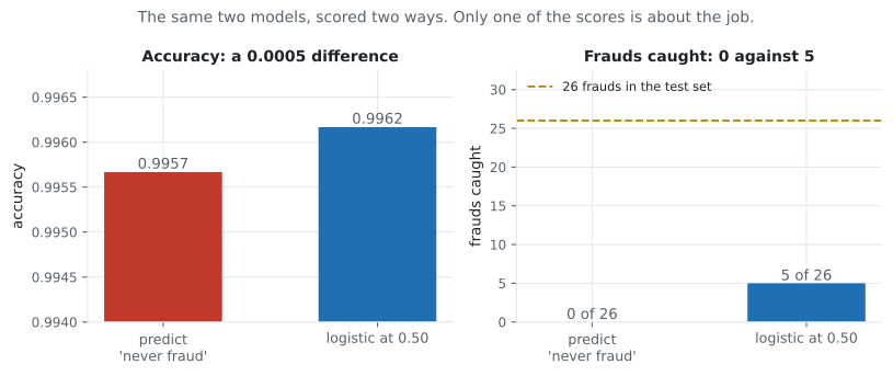
What you’ll learn

• why 0.9957 accuracy is the worst possible model on this dataset
• why ROC-AUC 0.9848 and average precision 0.4561 describe the same predictions
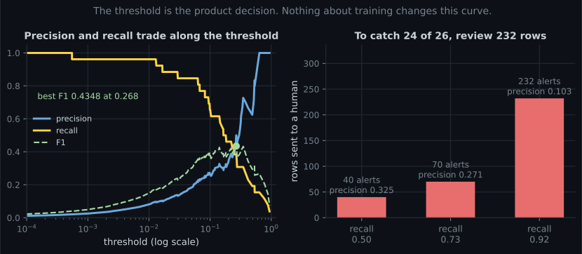
• how to pick a threshold from a recall target, and what it costs: 232 alerts to catch 24 of 26
• SMOTE implemented from its definition, in fifteen lines of numpy
• the measured verdict on resampling: no ranking improvement, and calibration destroyed
• the leakage that makes SMOTE look brilliant — 0.9879 against an honest 0.4517

The dataset

20,000 transactions, six features, and a label drawn from a logistic model whose intercept is solved so the fraud rate lands at 0.5%. Nothing is separable — the Bayes-optimal classifier still makes mistakes — which is what makes every question below non-trivial.

rng = np.random.default_rng(0)
X = rng.normal(0, 1, (20_000, 6))
w = np.array([1.4, 0.9, -1.1, 1.6, 2.0, 0.0])      # the last feature is noise
 
lo, hi = -30.0, 10.0                                # solve for a 0.5% base rate
for _ in range(200):
    mid = (lo + hi) / 2
    if sigmoid(X @ w + mid).mean() > 0.005:
        hi = mid
    else:
        lo = mid
 
p_true = sigmoid(X @ w + (lo + hi) / 2)
y = (rng.random(20_000) < p_true).astype(int)
 
print(y.sum(), y.mean())        # 87 0.0043

rng = np.random.default_rng(0)
X = rng.normal(0, 1, (20_000, 6))
w = np.array([1.4, 0.9, -1.1, 1.6, 2.0, 0.0])      # the last feature is noise
 
lo, hi = -30.0, 10.0                                # solve for a 0.5% base rate
for _ in range(200):
    mid = (lo + hi) / 2
    if sigmoid(X @ w + mid).mean() > 0.005:
        hi = mid
    else:
        lo = mid
 
p_true = sigmoid(X @ w + (lo + hi) / 2)
y = (rng.random(20_000) < p_true).astype(int)
 
print(y.sum(), y.mean())        # 87 0.0043

87 frauds in 20,000 rows. A 70/30 split puts 26 of them in the test set, alongside 5,974 legitimate transactions. Keep those two numbers in mind; almost every surprise on this page is a consequence of the second being 230 times the first.

The accuracy paradox, measured

figureThe same two models, scored two waysmatplotlib

never_fraud = np.zeros(len(y_test), dtype=int)
print(f"{(never_fraud == y_test).mean():.4f}")      # 0.9957, catching 0 of 26
 
model = make_pipeline(StandardScaler(), LogisticRegression(max_iter=2000))
model.fit(X_train, y_train)
proba = model.predict_proba(X_test)[:, 1]
print(f"{((proba >= 0.5) == y_test).mean():.4f}")   # 0.9962, catching 5 of 26

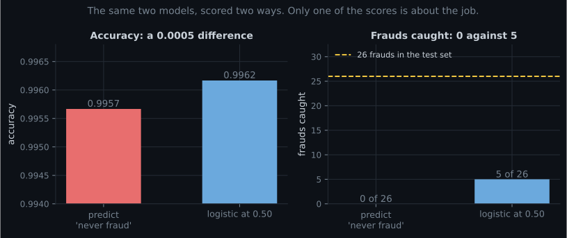
never_fraud = np.zeros(len(y_test), dtype=int)
print(f"{(never_fraud == y_test).mean():.4f}")      # 0.9957, catching 0 of 26
 
model = make_pipeline(StandardScaler(), LogisticRegression(max_iter=2000))
model.fit(X_train, y_train)
proba = model.predict_proba(X_test)[:, 1]
print(f"{((proba >= 0.5) == y_test).mean():.4f}")   # 0.9962, catching 5 of 26

A model that has never heard of fraud scores 0.9957. The fitted model — which happens to be the correct model, since the data was generated by a logistic rule — scores 0.9962 at the default threshold, and catches 5 of 26 with 2 false positives.

Accuracy is not merely uninformative here, it is actively misleading: it puts a 0.0005 gap between “nothing” and “something”, and it would put a similarly trivial gap between two genuinely different fraud systems.

ROC-AUC against average precision

Both are threshold-free summaries of the same ranking. They disagree violently.

figureOne set of predictions, two summaries: AUC 0.9848 and AP 0.4561matplotlib

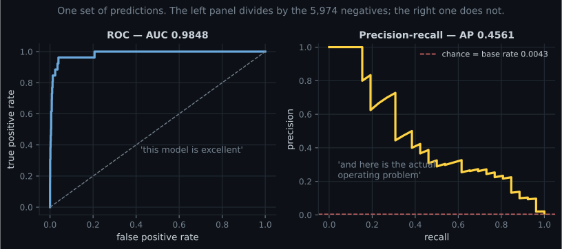
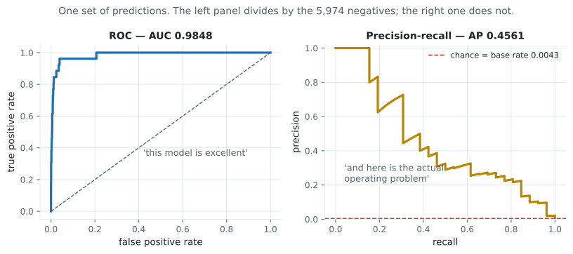
The mechanism is in the denominators:

FPR divides false positives by the 5,974 negatives, so 208 of them is 0.0348 — invisible on an ROC plot. Precision divides the same 208 by the 232 alerts, giving 0.1034. The negatives dominate one denominator and are absent from the other.

Average precision at 0.4561 against a 0.0043 baseline is a genuinely strong model — a 105× lift. It is also nowhere near 0.9848, and if you promised stakeholders “98%” you have promised something that does not exist.

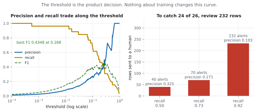
The threshold is the product decision

Nothing in training changes the trade-off below. It is a property of the ranking, and choosing a point on it is a business decision about how many humans you employ.

figureEach recall target has a price, quoted in rows a human must readmatplotlib

Read the last row carefully. Going from 19 to 24 frauds caught costs 162 extra reviews, and takes precision from 0.271 to 0.103. Whether that is a good trade depends on two numbers the model does not know: the average loss per undetected fraud, and the cost of a review. That calculation is the subject of the next page.

Note also what the F1-optimal threshold does. Best F1 is 0.4348 at threshold 0.268, giving precision 0.500 and recall 0.385 — it catches 10 of 26 frauds. F1 weights precision and recall equally, which is a statement about the world that is almost never true for fraud.

See it move

Precision under a rare event is bounded by arithmetic, not by model quality. Below, fraud scores are $\mathcal{N}(2, 1)$ and legitimate scores $\mathcal{N}(0,1)$ — a genuinely strong separation — and the base rate is yours to set. Everything is computed in closed form from the normal CDF.

Two invariants worth internalising. Recall does not depend on the base rate at all — it is a property of the positive class’s score distribution. Precision depends on it almost entirely: at 1 in 10 the same threshold gives comfortable precision, and at 1 in 10,000 the same model at the same threshold drowns in false alerts. When someone reports a fraud model’s precision, the first question is what base rate it was measured at.

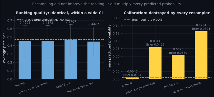
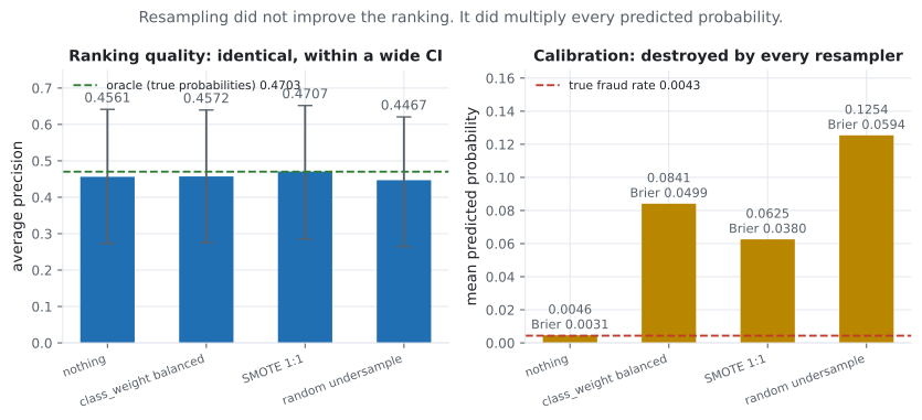
Resampling: what it actually does

The standard advice is to rebalance the training set. Four strategies on identical data, with a bootstrap confidence interval on average precision so the differences can be judged rather than admired:

figureNo ranking gain, and every resampler inflates the probabilitiesmatplotlib

Three readings, in order of importance.

The differences are noise. Every interval spans roughly 0.37 of average precision, from about 0.27 to 0.65. With 26 positives in the test set, an AP difference of 0.02 carries no information. Any blog post that reports “SMOTE improved AP from 0.456 to 0.471” on a test set this size is reporting sampling variation.

There was no headroom anyway. The oracle — scoring with the true probabilities that generated the labels — gets 0.4703. The plain model is already at the ceiling. No resampler can beat the data-generating process, and on a well-specified model none of them will.

Calibration is destroyed, and that is not noise. Mean predicted probability goes from 0.0046 against a true 0.0043, to 0.0841, 0.0625 and 0.1254. The Brier score degrades from 0.0031 to 0.0594. Resampling changes the prior the model was fit under, so every probability it outputs is a probability for a world where fraud happens 50% of the time.

If you need probabilities — and you do, the moment anyone multiplies them by a euro amount — this matters far more than the AP that did not move.

Correcting the prior back

If you do undersample, the shift is analytic. With a training positive rate of $\pi'$ and a true rate $\pi$, the corrected odds are

so a single multiplication on the odds scale undoes the sampling. Applied to the undersampled model — trained at $\pi' = 0.5$ against a true $\pi = 0.0044$ — it brings mean predicted probability from 0.1254 to 0.0031 against a true test rate of 0.0043, and the Brier score from 0.0594 to 0.0033. Average precision is unchanged at 0.4467, because the correction is monotone and cannot reorder anything.

That is why undersampling is the defensible resampler: its distortion is one known multiplication. SMOTE’s synthetic neighbours have no such closed-form undo.

SMOTE in fifteen lines

Worth writing once, because the mechanism explains both what it fixes and what it breaks.

def smote(X, y, k=5, seed=0):
    """Interpolate between a minority row and one of its k minority neighbours."""
    rng = np.random.default_rng(seed)
    X = np.asarray(X, dtype=float)
    minority = X[y == 1]
    n_needed = int((y == 0).sum()) - len(minority)      # grow to 1:1
 
    d = np.linalg.norm(minority[:, None, :] - minority[None, :, :], axis=2)
    np.fill_diagonal(d, np.inf)
    neighbours = np.argsort(d, axis=1)[:, :k]
 
    seeds = rng.integers(0, len(minority), n_needed)
    picks = neighbours[seeds, rng.integers(0, k, n_needed)]
    gaps = rng.random((n_needed, 1))
    synthetic = minority[seeds] + gaps * (minority[picks] - minority[seeds])
 
    return (np.vstack([X, synthetic]),
            np.concatenate([np.asarray(y), np.ones(n_needed, dtype=int)]))

def smote(X, y, k=5, seed=0):
    """Interpolate between a minority row and one of its k minority neighbours."""
    rng = np.random.default_rng(seed)
    X = np.asarray(X, dtype=float)
    minority = X[y == 1]
    n_needed = int((y == 0).sum()) - len(minority)      # grow to 1:1
 
    d = np.linalg.norm(minority[:, None, :] - minority[None, :, :], axis=2)
    np.fill_diagonal(d, np.inf)
    neighbours = np.argsort(d, axis=1)[:, :k]
 
    seeds = rng.integers(0, len(minority), n_needed)
    picks = neighbours[seeds, rng.integers(0, k, n_needed)]
    gaps = rng.random((n_needed, 1))
    synthetic = minority[seeds] + gaps * (minority[picks] - minority[seeds])
 
    return (np.vstack([X, synthetic]),
            np.concatenate([np.asarray(y), np.ones(n_needed, dtype=int)]))

Every synthetic row is a convex combination of two real minority rows. Three consequences follow directly:

• It cannot invent structure. Synthetic points lie on segments between existing ones, so SMOTE interpolates the minority cloud and never extrapolates beyond its convex hull.
• It amplifies mislabelled positives. A minority point that is actually a mistake becomes the parent of dozens of synthetic points.
• It is meaningless for categoricals. The midpoint of country=DEcountry=DE and country=BRcountry=BR is not a country. (SMOTE-NC exists and picks the majority category instead; know which variant you are running.)

Here it grew 61 minority rows into 13,939 of them — 228 synthetic points per real fraud, all of them inside the convex hull of 61 observations.

The leakage that makes it look brilliant

This is the single most common mistake in imbalanced-learning write-ups, and the numbers it produces are spectacular.

figure0.9879 against 0.4517, from the same fitted modelmatplotlib

# WRONG — synthetic rows built from training frauds end up in the test set
X_all, y_all = smote(X, y)
X_tr, X_te, y_tr, y_te = train_test_split(X_all, y_all, test_size=0.3)
# average precision: 0.9879
 
# The same fitted model, scored on the real test set: 0.4517

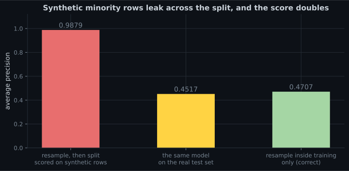
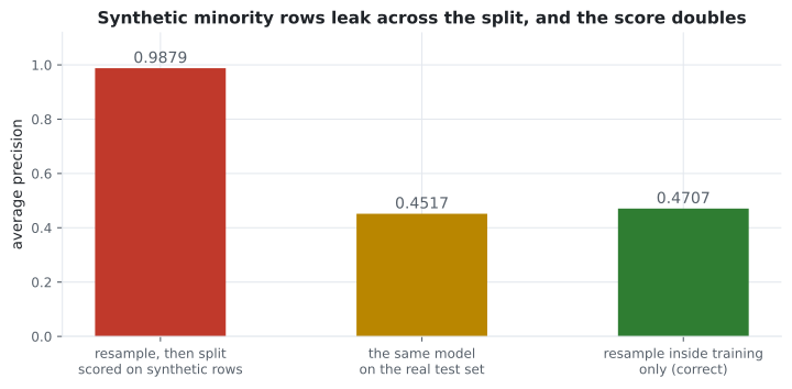
# WRONG — synthetic rows built from training frauds end up in the test set
X_all, y_all = smote(X, y)
X_tr, X_te, y_tr, y_te = train_test_split(X_all, y_all, test_size=0.3)
# average precision: 0.9879
 
# The same fitted model, scored on the real test set: 0.4517

The synthetic test rows are convex combinations of training frauds, so predicting them is nearly free. The reported 0.9879 is a measurement of interpolation, not of fraud detection.

The rule is mechanical: every resampling step belongs inside the training fold, which means inside each cross-validation split, which in practice means inside a PipelinePipeline (or imblearnimblearn’s PipelinePipeline, which understands resamplers). If you resample before you split, you will get a beautiful number and a useless model.

The workflow that works

  flowchart TD
  A["Rare positives"] --> B["Measure with average precision
and precision at your alert budget.
NEVER accuracy."]
  B --> C["Fit the plain model first
no resampling, no class_weight"]
  C --> D{"Do you need
probabilities?"}
  D -->|"yes — money, expected loss"| E["Keep the plain model.
Check calibration."]
  D -->|"no — only a ranking"| F["class_weight or resampling
are allowed, inside the fold"]
  E --> G["Choose the threshold from
the cost of each error"]
  F --> G
  G --> H["Report precision, recall AND
alerts per day at that threshold"]
  H --> I{"Not good enough?"}
  I -->|"no"| J["Better features
or more positives.
Not a different sampler."]
  I -->|"yes"| K["Ship, and monitor
the alert volume"]

The step people skip is the second one. Fitting the plain model first tells you whether there is a problem to solve: here it reached the oracle’s ceiling immediately, and every hour spent on samplers after that was an hour spent on nothing.

Pitfalls

Recap

• 87 frauds in 20,000 rows; 26 in the test set against 5,974 negatives.
• Predicting “never fraud” scores 0.9957. The correct model scores 0.9962 and catches 5 of 26.
• ROC-AUC 0.9848, average precision 0.4561 — the same predictions, a 105× lift over the 0.0043 chance line.
• Threshold sets the workload: 40 alerts for recall 0.50, 232 for recall 0.92 at precision 0.103.
• Four rebalancing strategies land within 0.024 AP of each other, with CIs spanning ~0.37, all at the oracle’s 0.4703 ceiling.
• Every resampler wrecks calibration: mean $\hat{p}$ up to 0.1254 against a true 0.0043, Brier 0.0031 → 0.0594.
• SMOTE before the split reports 0.9879; the same model scores 0.4517 honestly.

🧪 Try It Yourself

Exercise 1 – Build the rare-event dataset

Exercise 2 – Two metrics, one ranking

Exercise 3 – Price each recall target

Exercise 4 – SMOTE from scratch, and what it costs

Exercise 5 – Reproduce the leakage

Next

Cost-Sensitive Learning and Decision Thresholds — this page priced recall in alerts. The next one prices it in money, and derives the threshold that minimises expected loss instead of guessing at 0.5.