Q-Learning & Deep Q-Networks

Tabular Q-learning is a lookup table with one number per state-action pair, updated by a rule that provably converges. A Deep Q-Network is the same rule with a neural network in place of the table — and that substitution breaks the convergence guarantee outright.

Two mechanisms exist to patch it: experience replay and a target network. Both are usually presented as sensible ideas. Here they are ablated on CartPole, three seeds each:

Configuration	Final episode length	sd	Worst seed	Best seed
Replay + target	144.20	7.91	136.82	155.17
Replay only	53.45	1.84	51.98	56.05
Target only	53.45	36.58	25.47	105.12
Neither	48.81	10.50	40.32	63.60
Random policy	23.09	—	—	—

Neither mechanism does much alone — 53.45 either way, against 48.81 for nothing at all. Together they reach 144.20. The interesting row is target only, whose seeds ranged from 25.47 (barely better than random) to 105.12.

What you’ll learn

• The Q-learning update, and the one property that makes the tabular version safe.
• Why replacing the table with a network breaks it, in two distinct ways.
• What replay and the target network each fix, measured by ablation.
• Why a learning rate of 1.0 destroys tabular learning in a stochastic world — reward −1.6025, goal rate 0.0100.

The update

$$Q(s, a) \leftarrow Q(s, a) + \alpha\Big[\underbrace{r + \gamma \max_{a'} Q(s', a')}_{\text{target}} - Q(s, a)\Big]$$

The bracket is a temporal-difference error: the difference between what we thought this state-action was worth and what one step of real experience suggests. The tabular version is safe because each entry is independent — updating $Q(s, a)$ changes nothing else.

That independence is exactly what a network destroys. Every weight update changes the predicted value of every state, including the $s'$ used to compute the target.

Learning rate and exploration, on the gridworld

Before adding a network, here is the tabular version on the stochastic gridworld from the previous page, where value iteration scores 0.6849 reward with a 0.9033 goal rate:

figure 3,000 episodes per cell, greedy evaluation over 300 episodes matplotlib

A learning rate of 1.0 means each update throws away the old estimate entirely and believes the single most recent transition. In a world where actions slip 15% of the time, that single transition is often unrepresentative, and the table never settles — reward -1.6025 with a goal rate of 0.0100, far worse than random wandering. The best cell measured was alpha 0.05 with epsilon 0.10, at 0.6951.

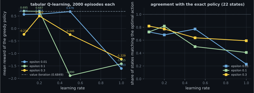
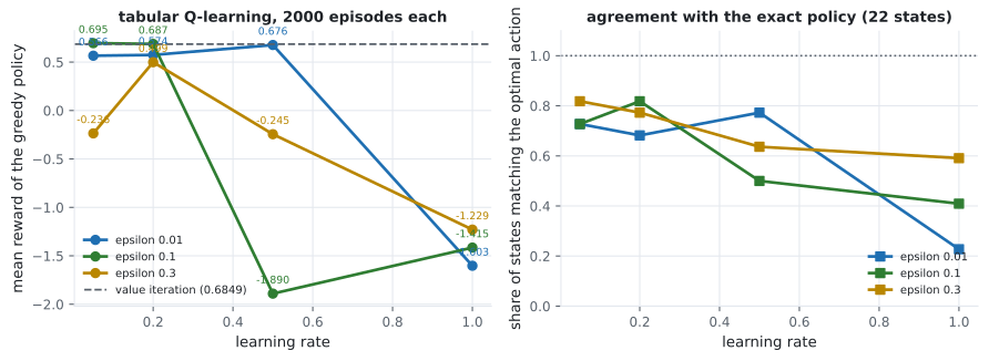
α	ε	Reward	Goal rate	Policy match
0.05	0.10	0.6951	0.9133	0.7273
0.20	0.10	0.6872	0.9067	0.8182
0.50	0.01	0.6765	0.9033	0.7727
0.50	0.10	−1.8901	0.0200	0.5000
1.00	0.01	−1.6025	0.0100	0.2273
1.00	0.30	−1.2294	0.1633	0.5909

Two things worth noticing. First, the α = 0.50, ε = 0.10 cell scored −1.8901 while its neighbours at α = 0.50 scored 0.6765 and 0.4990 — a single unlucky combination, which is a reminder that each cell here is one run, not an average. Second, policy match never exceeds 0.8182: even the best runs disagree with the optimal policy on a fifth of states, because ε-greedy rarely visits the safe corridor.

Why a network breaks it

diagram Diagram mermaid

  flowchart TD
  T["tabular Q-learning"] --> I["each entry independent"]
  I --> C["converges"]
  N["network Q-learning"] --> P1["one update changes
every state's value"]
  N --> P2["consecutive samples
are highly correlated"]
  P1 --> B["the target moves
while you fit it"]
  P2 --> D["gradient steps on
near-duplicate data"]
  B -->|"fix: target network"| F1["freeze a copy for 200 frames"]
  D -->|"fix: experience replay"| F2["sample from a 10k buffer"]
  F1 --> R["144.20 together"]
  F2 --> R

Correlated samples. Consecutive CartPole states differ by one 0.02-second Euler step. A network fitted on a stream of them sees a hundred near-duplicates in a row, drifts to fit that narrow slice, and forgets the rest. Replay fixes this by keeping the last 10,000 transitions and sampling a random batch of 64.

A moving target. The regression target is $r + \gamma \max_{a'} Q(s', a')$, computed with the same network being updated. Fitting a target that shifts every time you fit it is not regression in any usual sense. The target network fixes this by scoring $s'$ with a frozen copy, refreshed every 200 frames.

The two mechanisms, in the lines that implement them

# Replay: a random batch from the buffer, not the last few transitions.
batch = rng.integers(0, filled, BATCH) if replay else recent_indices()
 
# Target network: score the next state with a frozen copy.
scorer = target_q if target_network else online_q
future = scorer(following[batch]).max(axis=1)
wanted = rewards[batch] + GAMMA * future * (1 - finished[batch])
 
current = online_q(states[batch])
current[np.arange(len(batch)), actions[batch]] = wanted
step(states[batch], current)                    # one gradient step
 
if target_network and frame % TARGET_SYNC == 0:
    target.set_weights(online.get_weights())

The ablation

figure 6,000 frames across 16 parallel environments, 3 seeds each matplotlib

The two mechanisms are not independently useful here — each alone lands at 53.45, barely above the 48.81 of using neither. Together they reach 144.20. The error bars carry the other half of the story: replay-only is remarkably consistent (sd 1.84) because it reliably plateaus, while target-only ranges from 25.47 to 105.12 depending on the seed.

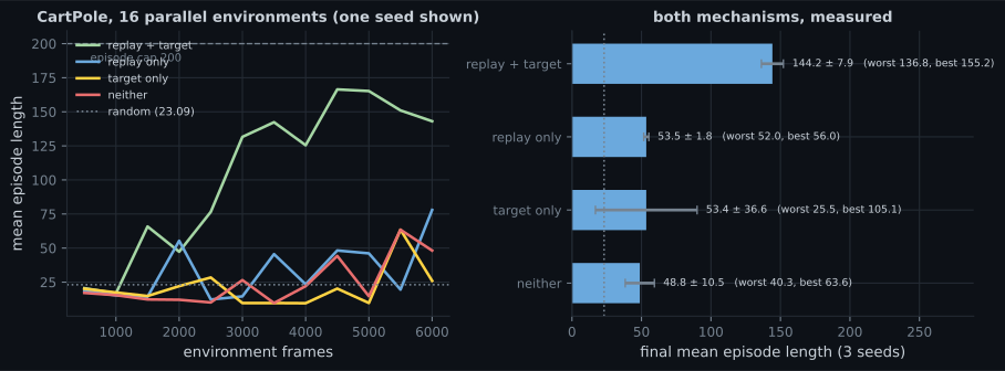
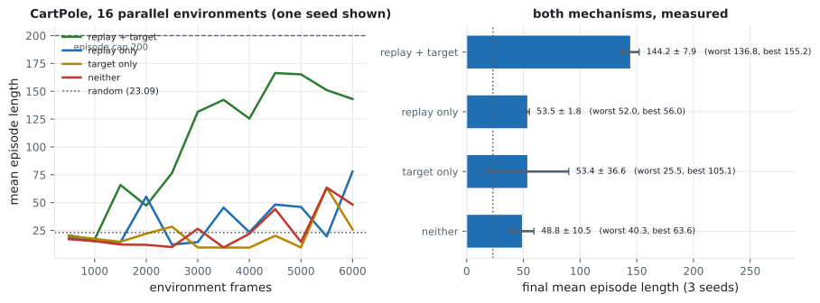
The pattern is worth stating carefully, because “both matter” is the easy reading and it understates the result. Each mechanism addresses a different failure, and fixing one while leaving the other in place leaves the agent broken by the one that remains:

• With replay but no target network, the data is decorrelated but the regression target still moves with every gradient step.
• With a target network but no replay, the target is stable but the network is being fitted on 64 near-identical consecutive transitions.

Only removing both obstacles produces learning, which is why DQN is usually described as needing both — and why the measured 53.45 / 53.45 / 48.81 cluster is more informative than the headline 144.20.

What the learned values look like

figure Tabular Q-learning against value iteration, gridworld matplotlib

The mean signed error is -0.1273 — the learned values UNDERESTIMATE the true ones. Textbooks predict the opposite, because the max in the update is taken over noisy estimates and so tends to select overestimates. That bias is real, but here it is swamped by a larger effect: epsilon-greedy rarely visits the safe corridor, so those states keep values learned from too few visits.

When the textbook prediction does not reproduce

Maximisation bias is the standard motivation for Double DQN, which decouples choosing the best action from evaluating it. The effect is genuine — taking a max over noisy estimates does select for the ones that happened to be too high — but it is not the dominant error in every setting. Here, under-exploration produced a net under-estimate of −0.1273.

Reporting the measured sign rather than the expected one is the whole point of running the experiment.

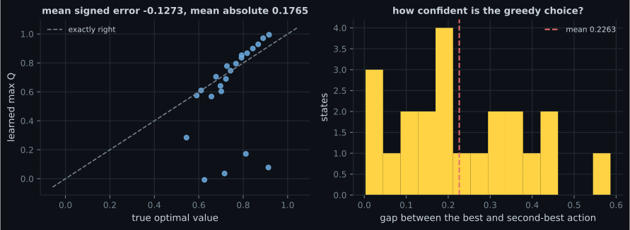
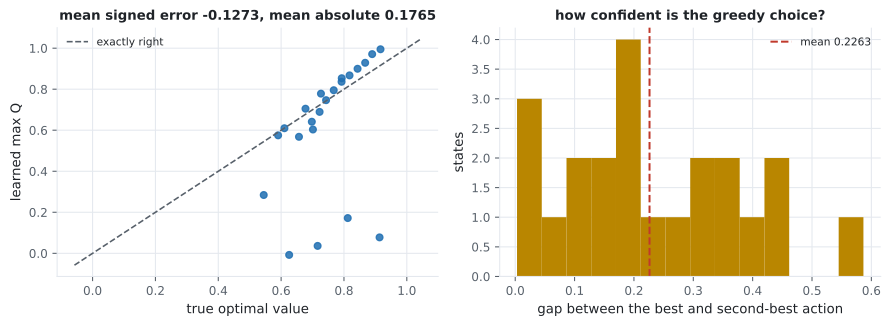
The right-hand histogram matters for a different reason: it shows how close the best and second-best actions usually are. In states where that gap is small, a tiny estimation error flips the greedy action, which is why policy match tops out at 0.8182 even when the values themselves are roughly right.

sketch The moving target problem p5.js Pause Restart

Step the two fitting processes and watch the difference. On the left the target moves with the estimate; on the right it is frozen and refreshed periodically.

sketch The measured table, ranked p5.js Pause Restart

Click a column to rank every row by it. The bars are that column's values and the highest and lowest are computed from the numbers, not written in.

Pitfalls

• Using a high learning rate in a stochastic environment. α = 1.0 replaces the estimate with the latest transition, and scored −1.6025 with a 0.0100 goal rate.
• Adding replay or a target network alone and concluding it did not help. Each scored 53.45; together they scored 144.20.
• Reading a single seed. Target-only ranged from 25.47 to 105.12 across three seeds.
• Assuming learned Q-values overestimate. Measured here at −0.1273, because under-exploration outweighed maximisation bias.
• Judging a policy by value accuracy. Policy match peaked at 0.8182 even where the values were close, because many states have a tiny gap between the best and second-best action.
• Calling predict() inside the loop. Measured at roughly 470ms per call against 1.2ms for a traced tf.function — an RL loop makes several calls per frame.
• Treating a time-limit ending as a terminal state. This implementation does, which is the standard simplification, and it slightly under-values states near the 200-step cap.

Recap

• Q-learning updates towards $r + \gamma \max_{a'} Q(s', a')$; the tabular version is safe because entries are independent.
• A network couples every state to every other, which breaks that independence in two ways: correlated samples and a moving target.
• Replay and a target network fix one each, and measured alone neither was enough — 53.45 and 53.45, against 48.81 for neither and 144.20 for both.
• In the tabular world, α = 0.05 with ε = 0.10 was best (0.6951); α = 1.0 collapsed to −1.6025.
• Learned values underestimated the optimum by 0.1273 on average, the opposite of the textbook prediction, because exploration was the larger error source.
• Policy match never exceeded 0.8182, since small value errors flip the greedy action wherever two actions are close.

Next

DQN learns a value and derives a policy from it. The alternative is to skip the value function and adjust the policy directly, which trades one problem for a noisier one: Policy Gradients (Intro).

pch.quizTag pch.quizDefaultTitle

1. Replay alone scored 53.45, a target network alone scored 53.45, and both together scored 144.20. What does that show?

   A The two mechanisms are redundant B They fix different failures — correlated samples and a moving regression target — so removing one obstacle while leaving the other still leaves the agent broken by the remaining one C The target network is unnecessary D The measurements are within noise of each other
   pch.quizShowAnswer

   B — They fix different failures — correlated samples and a moving regression target — so removing one obstacle while leaving the other still leaves the agent broken by the remaining one — Both-together is nearly three times either-alone, and either-alone is barely above the 48.81 of using neither.

2. Why does replacing a Q-table with a network break Q-learning's convergence guarantee?

   A Networks are not expressive enough B The table's entries are independent, so updating one changes nothing else; a network's weights are shared, so every update changes the predicted value of every state including the one used to build the target C Gradient descent cannot minimise a temporal-difference error D Because the reward becomes stochastic
   pch.quizShowAnswer

   B — The table's entries are independent, so updating one changes nothing else; a network's weights are shared, so every update changes the predicted value of every state including the one used to build the target — That shared-parameter coupling is precisely what the target network works around, by freezing a copy to compute targets with.

3. Tabular Q-learning with a learning rate of 1.0 scored -1.6025 with a goal rate of 0.0100, worse than random. Why?

   A The learning rate caused numerical overflow B Alpha 1.0 discards the running estimate and adopts the single most recent transition — and in a world where actions slip 15% of the time, that transition is frequently unrepresentative, so the table never settles C It converged to a local optimum D It needed more episodes
   pch.quizShowAnswer

   B — Alpha 1.0 discards the running estimate and adopts the single most recent transition — and in a world where actions slip 15% of the time, that transition is frequently unrepresentative, so the table never settles — In a deterministic world alpha 1.0 is harmless. The failure is specific to stochastic transitions.

4. The learned Q-values had a mean signed error of -0.1273 against the exact values, while the textbook predicts overestimation. What is the honest interpretation?

   A The measurement is wrong B Maximisation bias is real but was not the dominant error here — epsilon-greedy rarely visited the safe corridor, so those states retained values learned from too few visits, producing a net underestimate C Double DQN is unnecessary D The exact values were computed incorrectly
   pch.quizShowAnswer

   B — Maximisation bias is real but was not the dominant error here — epsilon-greedy rarely visited the safe corridor, so those states retained values learned from too few visits, producing a net underestimate — Reporting the measured sign rather than the expected one is the reason for running the experiment at all.

5. Even the best tabular run matched the optimal policy in only 0.8182 of states, despite scoring near-optimal reward. How can both be true?

   A The reward measurement is unreliable B Many states have a very small gap between the best and second-best action, so a tiny value error flips the greedy choice without costing much reward C Policy match is computed on terminal states too D The evaluation used too few episodes
   pch.quizShowAnswer

   B — Many states have a very small gap between the best and second-best action, so a tiny value error flips the greedy choice without costing much reward — The histogram of best-minus-second-best action values is concentrated near zero, which is exactly the condition for this to happen.

🧪 Try It Yourself

pch.exerciseTag pch.exerciseTitle

pch.exerciseTag pch.exerciseTitle

pch.exerciseTag pch.exerciseTitle

pch.exerciseTag pch.exerciseTitle

pch.exerciseTag pch.exerciseTitle

pch.exerciseTag pch.exerciseTitle