Neural Style Transfer

DeepDream optimised an image to maximise one number. Style transfer keeps that machinery — frozen network, image as the variable — and replaces the objective with a comparison against two reference images:

$$\mathcal{L} = \underbrace{\sum_{\ell \in C} \lVert F^\ell(x) - F^\ell(c) \rVert^2}_{\text{content}} + w \cdot \underbrace{\sum_{\ell \in S} \lVert G^\ell(x) - G^\ell(s) \rVert^2}_{\text{style}}$$

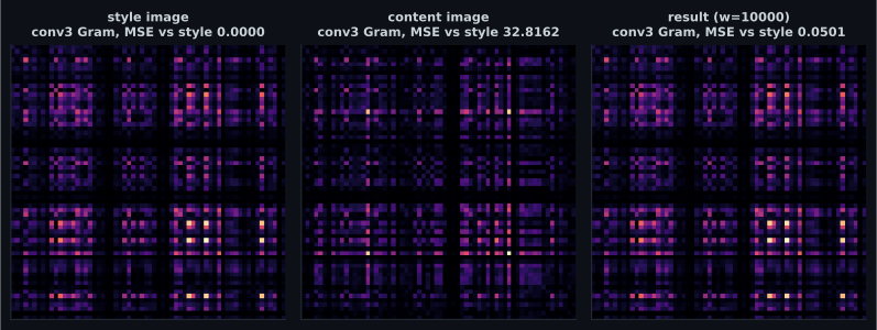
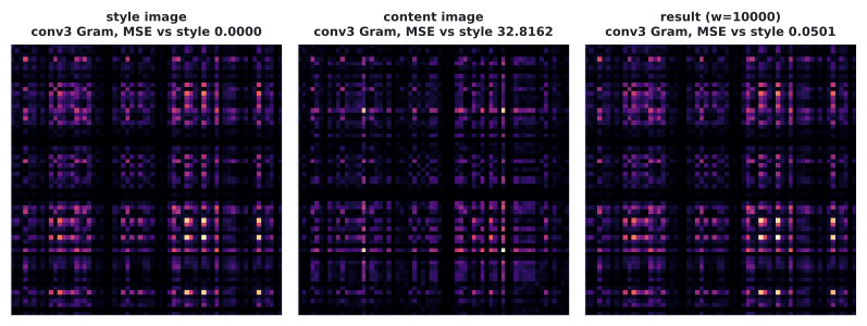
Content is compared activation by activation, so layout is preserved. Style is compared through the Gram matrix $G$, which throws away position and keeps only how features co-occur — which is precisely why it transfers texture without transferring the subject.

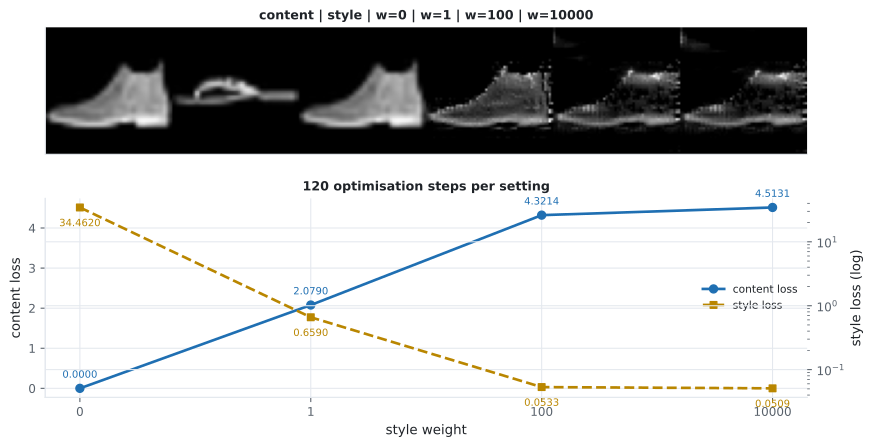
The weight $w$ between those terms is the only interesting hyperparameter, and it trades one term against the other exactly as you would hope, measured over 120 optimisation steps:

Style weight	Content loss	Style loss	Total objective
0	0.00000	34.46199	0.00000
1	2.07898	0.65903	2.73801
100	4.32142	0.05325	9.64647
10000	4.51310	0.05092	513.73618

(The totals come from the run’s full-precision losses; recomputing them from the rounded columns above gives 9.64642 and 513.71310.)

Style loss falls by a factor of 677 across that sweep while content loss rises from zero to 4.51310. There is no setting that improves both.

No pretrained weights here

Published style transfer uses VGG19 trained on ImageNet. Nothing pretrained is cached on this machine, so the features come from a small fully convolutional network trained here on Fashion-MNIST — 23,946 parameters, 0.7767 validation accuracy. The mechanism, the losses and every number are real; the transferable “style” is garment texture rather than brushwork, and a deeper feature network is what makes the famous results look the way they do.

What you’ll learn

• Why content uses raw activations and style uses the Gram matrix, and what discarding position buys.
• The measured trade across four style weights, including why weight 0 has a content loss of exactly zero.
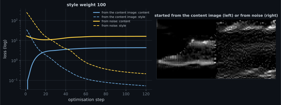
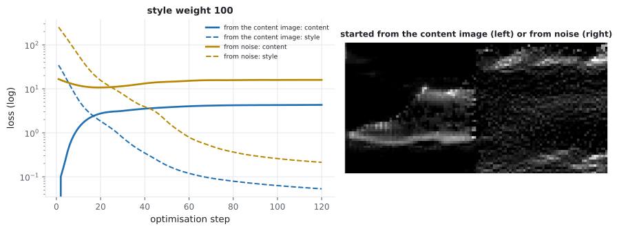
• Why the starting image is a real hyperparameter: starting from noise ended up worse on both terms (content 15.97160 against 4.32142).
• What “nothing is trained” means in code — one tf.Variable holding the image, and an optimiser applied to it.

The Gram matrix

For one layer’s activation of shape (height, width, channels), flatten the spatial dimensions and take the correlation between channels:

$$G_{ij} = \frac{1}{HW} \sum_{p} F_{pi} F_{pj}$$

Every spatial position $p$ is summed over, so the result says how often channel $i$ fires where channel $j$ fires and says nothing about where. A texture is exactly that: a statistical relationship between features, repeated across an image without a fixed layout.

Style is a correlation, not a picture

def gram(activation):
    shape = tf.shape(activation)
    flat = tf.reshape(activation, (shape[0], -1, shape[3]))   # positions x channels
    return tf.matmul(flat, flat, transpose_a=True) / tf.cast(shape[1] * shape[2],
                                                            "float32")

Dividing by the number of positions matters more than it looks: without it the Gram matrix scales with image area, so the style loss would depend on resolution and a weight tuned at one size would be wrong at another.

figure conv3 channel correlations, MSE against the style image matplotlib

These are the actual quantities the style loss compares. The result's Gram matrix has been optimised towards the style image's, and the middle panel shows how different the content image's correlations were to begin with — that difference is what the 34.46199 starting style loss measures.

diagram Diagram mermaid

  flowchart LR
  C["content image"] --> E1["frozen convnet"]
  S["style image"] --> E2["frozen convnet"]
  X["the image being optimised
(a tf.Variable)"] --> E3["frozen convnet"]
  E1 --> CT["conv3 activations"]
  E2 --> GT["Gram matrices
conv1, conv2, conv3"]
  E3 --> XA["activations + Gram"]
  CT --> L1["content loss"]
  GT --> L2["style loss"]
  XA --> L1
  XA --> L2
  L1 --> T["total = content + w * style"]
  L2 --> T
  T -->|"gradient with respect to the IMAGE"| X

Nothing is trained

The only variable is the image. This is worth writing out, because it is the part that surprises people who have only ever called model.fit:

The image is the parameter

variable = tf.Variable(initial_image)              # <- the only trainable thing
optimizer = keras.optimizers.Adam(0.02)
 
for _ in range(STEPS):
    with tf.GradientTape() as tape:
        named = dict(zip(names, extractor(variable)))
        content_loss = tf.reduce_mean((named["conv3"] - content_target) ** 2)
        style_loss = tf.add_n([tf.reduce_mean((gram(named[layer]) - target) ** 2)
                               for layer, target in style_targets.items()])
        loss = content_loss + style_weight * style_loss
 
    optimizer.apply_gradients([(tape.gradient(loss, variable), variable)])
    variable.assign(tf.clip_by_value(variable, 0.0, 1.0))   # keep pixels legal

The assign after each step is the equivalent of DeepDream’s clip: an optimiser will happily walk pixels outside the valid range, and the resulting image cannot be displayed even though its loss looks fine.

The style weight

figure 120 optimisation steps per setting matplotlib

At weight 0 the objective ignores style entirely, so the optimum is the content image itself and the content loss is exactly 0.00000 — that is the floor the other settings are measured against. The interesting region is narrow: between weight 1 and weight 100 the style loss falls from 0.65903 to 0.05325 while content loss doubles from 2.07898 to 4.32142, and past that, weight 10000 buys a further 0.00233 of style loss for 0.19168 more content loss.

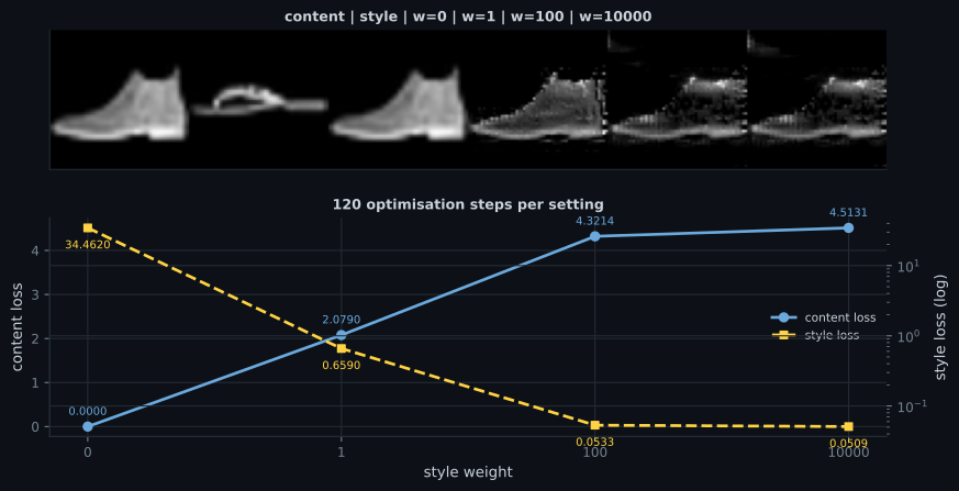
Reading the sweep as an engineering decision rather than a picture:

• Weight 0 is the control. The objective is content-only, the starting image is the content image, and the optimum is therefore to change nothing — content loss 0.00000, and a style loss of 34.46199, which is simply how far apart the two images’ correlations are to begin with.
• Weight 1 is where the trade is efficient. 94% of the available style-loss reduction (34.46199 → 0.65903) for 2.07898 of content loss.
• Weight 100 is past the knee. A further 0.60578 of style loss costs another 2.24244 of content.
• Weight 10000 is wasted. 0.00233 more style loss reduction for 0.19168 more content loss. The total objective is dominated so completely by the style term that the content gradient is effectively noise.

The diminishing returns are the point. Style loss is bounded below by zero and the run is already close to it at weight 100; content loss has no such limit, so it absorbs everything the larger weight demands.

Where you start from

Style transfer is a non-convex optimisation over a 3,136-dimensional image, so the starting point does not merely affect how long it takes — it selects which solution is found.

figure Both at style weight 100, 120 steps each matplotlib

Starting from noise is worse on BOTH terms at the same budget: content loss 15.97160 against 4.32142, and style loss 0.21332 against 0.05325. That is not a speed difference that more steps would erase — the two runs are descending into different basins, and the one that starts at the content image begins inside the region where the content term is already satisfied.

Starting image	Content loss	Style loss
The content image	4.32142	0.05325
Noise	15.97160	0.21332

The noise-started run is 3.70× worse on content and 4.01× worse on style. Published style transfer implementations almost always initialise from the content image, and this is why — it is not a convenience, it is a better optimum at equal cost.

sketch Content against style p5.js Pause Restart

Drag the slider to set the style weight. The bars show the two loss terms measured on this page, and the total the optimiser actually minimises.

sketch The measured table, ranked p5.js Pause Restart

Click a column to rank every row by it. The bars are that column's values and the highest and lowest are computed from the numbers, not written in.

Pitfalls

• Not normalising the Gram matrix by the number of positions. It would then scale with image area, so a style weight tuned at one resolution would be wrong at another.
• Expecting one weight to improve both terms. Style loss fell 677× across the sweep and content loss rose monotonically; there is no free setting.
• Pushing the style weight higher and expecting more style. From 100 to 10000, style loss improved by 0.00233 while content loss rose 0.19168.
• Starting from noise. At equal budget it was worse on both terms — 15.97160 and 0.21332 against 4.32142 and 0.05325.
• Forgetting to clip the variable after each step. The optimiser will move pixels out of range and the loss will not complain.
• Comparing loss values across implementations. These depend on the feature network (0.7767 accuracy here), which layers were chosen, and the Gram normalisation.
• Using a single style layer. Style is a multi-scale property; the three layers used here contribute correlations at three different receptive-field sizes.

Recap

• Style transfer optimises the image against a frozen network — nothing is trained.
• Content loss compares activations directly; style loss compares Gram matrices, which discard position and keep feature co-occurrence.
• The measured trade over 120 steps: style loss 34.46199 → 0.05092 while content loss 0.00000 → 4.51310.
• Weight 0 gives content loss exactly 0.00000, because the content image is both the start and the optimum — the floor everything else is measured against.
• Returns diminish sharply: weight 1 captured 94% of the available style reduction, and weight 10000 bought 0.00233 more for 0.19168 of content loss.
• The starting image selects the basin: from noise, both terms ended worse (15.97160 and 0.21332).

Next

That completes the generative phase — six families, all measured against baselines rather than admired. The phase summary collects what each one cost and what it actually produced: Phase 6 - Generative Deep Learning.

pch.quizTag pch.quizDefaultTitle

1. Why does style loss use the Gram matrix rather than comparing activations directly?

   A Because it is cheaper to compute B Because summing over all spatial positions discards WHERE features fired and keeps only how they co-occur — which is what a texture is, and what lets style transfer without transferring the subject C Because activations are too noisy D Because the Gram matrix is differentiable and activations are not
   pch.quizShowAnswer

   B — Because summing over all spatial positions discards WHERE features fired and keeps only how they co-occur — which is what a texture is, and what lets style transfer without transferring the subject — Content loss deliberately does the opposite: it compares activations position by position, which is what preserves layout.

2. At style weight 0 the content loss was exactly 0.00000. Why?

   A The optimiser failed to run B The objective was content-only and the run started from the content image, so the optimum is to change nothing — which makes it the floor that every other weight is measured against C The content loss is always zero at the first step D The style image happened to match the content image
   pch.quizShowAnswer

   B — The objective was content-only and the run started from the content image, so the optimum is to change nothing — which makes it the floor that every other weight is measured against — Its style loss of 34.46199 is also informative: that is how far apart the two images' feature correlations are before any optimisation.

3. Raising the style weight from 100 to 10000 reduced style loss by 0.00233 and raised content loss by 0.19168. What does that indicate?

   A The higher weight is better because style is the goal B Diminishing returns — style loss is bounded below by zero and was already near it, while content loss has no such bound, so the extra weight buys almost nothing at real cost C The optimisation diverged D The Gram matrix was not normalised
   pch.quizShowAnswer

   B — Diminishing returns — style loss is bounded below by zero and was already near it, while content loss has no such bound, so the extra weight buys almost nothing at real cost — The total objective at weight 10000 is dominated so heavily by the style term that the content gradient is effectively noise.

4. Starting from noise instead of the content image gave content loss 15.97160 against 4.32142 and style loss 0.21332 against 0.05325, at the same step budget. What is the conclusion?

   A The noise run just needs more steps to catch up B The optimisation is non-convex, so the starting point selects which solution is found — the two runs descended into different basins, and the noise run was worse on both terms C Noise initialisation always fails D The style weight was too low for the noise run
   pch.quizShowAnswer

   B — The optimisation is non-convex, so the starting point selects which solution is found — the two runs descended into different basins, and the noise run was worse on both terms — Being worse on both terms at once is the signature of a different basin rather than of slower progress along the same path.

5. What is actually being trained during style transfer?

   A The last layer of the feature network B Nothing — the image itself is a tf.Variable and the optimiser updates its pixels, while the network's weights stay frozen C A small generator network D The Gram matrices
   pch.quizShowAnswer

   B — Nothing — the image itself is a tf.Variable and the optimiser updates its pixels, while the network's weights stay frozen — This is the same pattern as DeepDream: a frozen network, an image as the parameter, and gradient steps on a differentiable objective.

🧪 Try It Yourself

pch.exerciseTag pch.exerciseTitle

pch.exerciseTag pch.exerciseTitle

pch.exerciseTag pch.exerciseTitle

pch.exerciseTag pch.exerciseTitle

pch.exerciseTag pch.exerciseTitle

pch.exerciseTag pch.exerciseTitle