What you’ll learn

• the two equivalent definitions of PCA — maximise variance and minimise reconstruction error — and why they are the same optimisation
• a complete eigendecomposition by hand on five points, matching scikit-learn exactly
• the SVD route, and why scikit-learn takes it instead of forming the covariance matrix
• explained variance ratio and how to pick $d$: digits needs 21 of 64 for 90%
• the standardisation failure, measured: PC1 at 99.8% and it is one column’s units
• reconstruction, compression and denoising with inverse_transforminverse_transform
• randomised and incremental PCA, and Kernel PCA for curved structure

Intuition

A dataset with 64 columns does not usually have 64 independent things going on. Neighbouring pixels in an image move together. Height and weight move together. Most of the columns are echoes of a smaller number of underlying factors.

PCA finds those factors. It looks for the direction in which the data spreads out the most, calls that the first principal component, then looks for the direction of greatest remaining spread that is perpendicular to the first, and so on. Keep the first few and you have a compact description that loses very little.

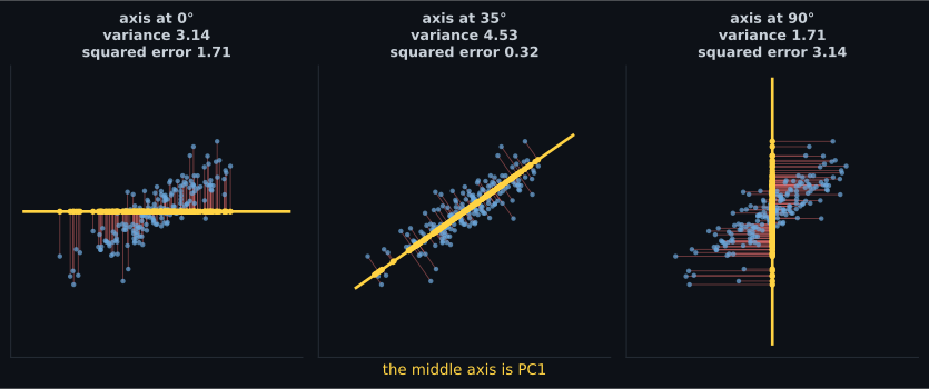
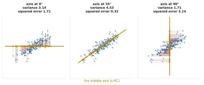
There are two ways to say what PCA optimises, and they turn out to be the same thing:

1. Maximise the variance of the projected data.
2. Minimise the squared distance from each point to its projection.

The reason is Pythagoras. For centred data, each point’s squared distance from the origin splits exactly into the squared length of its projection plus the squared length of the residual:

Summed over all points, the left side is a constant of the data. So maximising the first term is identical to minimising the second. Variance kept and error made are two names for one number.

  flowchart LR
  X["X (n x p)"] --> C["Centre each column
(and standardise)"]
  C --> S["SVD: X = U S V'"]
  S --> V["Components = rows of V'
Eigenvalues = s^2 / (n-1)"]
  V --> Z["transform: Z = Xc @ V
(n x d)"]
  Z --> R["inverse_transform:
Z @ V' + mean"]
  R --> E["Error = the variance in the
p - d discarded directions"]

figureThree candidate axes, one optimummatplotlib

The math

Let $\mathbf{X}$ be the $n \times p$ data matrix with every column already centred (PCA subtracts the mean for you; the derivation requires it). The sample covariance matrix is

For a unit direction $\mathbf{u}$, the projected values are $\mathbf{X}\mathbf{u}$ and their variance is

So PCA is the constrained problem

The constraint matters: without it you could inflate the objective forever by lengthening $\mathbf{u}$. Form the Lagrangian

and differentiate:

The optimum is an eigenvector of the covariance matrix. Left-multiplying by $\mathbf{u}^\top$ gives $\mathbf{u}^\top\mathbf{C}\mathbf{u} = \lambda$, so the variance captured by a component is its eigenvalue. Take the eigenvectors in descending order of $\lambda$ and you have the principal components.

Because $\mathbf{C}$ is real and symmetric, the spectral theorem guarantees its eigenvalues are real and its eigenvectors can be chosen orthonormal. Orthogonality of the components is not a design choice — it falls out of the mathematics.

The explained variance ratio

The eigenvalues sum to the total variance, $\sum_j \lambda_j = \operatorname{tr}(\mathbf{C})$, so

is the fraction of total variance the $j$-th component carries.

The SVD route

scikit-learn does not build $\mathbf{C}$. It takes the singular value decomposition directly:

Then

so the right singular vectors $\mathbf{V}$ are the eigenvectors of $\mathbf{X}^\top\mathbf{X}$, and the eigenvalues are $\lambda_j = \sigma_j^2/(n-1)$.

Two reasons this is better. Numerically, forming $\mathbf{X}^\top\mathbf{X}$ squares the condition number, so information near the noise floor is destroyed before you start. Computationally, when $p \gg n$ — 10,000 genes and 200 patients — the covariance matrix is $10{,}000 \times 10{,}000$ while the SVD never forms it.

The sign of each component is arbitrary: if $\mathbf{u}$ is an eigenvector so is $-\mathbf{u}$. scikit-learn applies a deterministic sign convention so results are reproducible, but do not read meaning into whether a loading is positive or negative in isolation.

Worked example by hand

Five points:

Step 1 — centre. The means are $\bar{x} = 4$ and $\bar{y} = 3$:

Step 2 — covariance. With $n - 1 = 4$:

Step 3 — eigenvalues. Solve $\det(\mathbf{C} - \lambda \mathbf{I}) = 0$:

Check against the trace: $4.5 + 0.5 = 5.0 = 2.5 + 2.5$. ✓

Step 4 — eigenvectors. For $\lambda_1 = 4.5$:

Normalised: $\mathbf{u}_1 = (1/\sqrt{2},\ 1/\sqrt{2}) = (0.7071,\ 0.7071)$. The same algebra with $\lambda_2 = 0.5$ gives $\mathbf{u}_2 = (-0.7071,\ 0.7071)$, which is perpendicular, as promised.

Step 5 — explained variance.

Ninety percent of the variation lies along the $45°$ diagonal.

Step 6 — project. The score of a point is its centred coordinates dotted with $\mathbf{u}_1$. For $(2, 1)$, centred to $(-2, -2)$:

All five scores: $-2.8284,\ -0.7071,\ -0.7071,\ 2.1213,\ 2.1213$.

Step 7 — reconstruct. Push the first point back out: $-2.8284 \times (0.7071, 0.7071) = (-2, -2)$, add the mean, and you get exactly $(2, 1)$. That point lies on the diagonal, so nothing was lost. Across all five points, the total squared reconstruction error from one component is 2.0 — which is $(n-1)\lambda_2 = 4 \times 0.5$, the discarded eigenvalue, exactly as the theory says.

Every number here matches sklearn.decomposition.PCAsklearn.decomposition.PCA to the digit.

See it move

The next sketch shows the two objectives moving in lockstep — as one bar rises, the other falls by exactly the same amount.

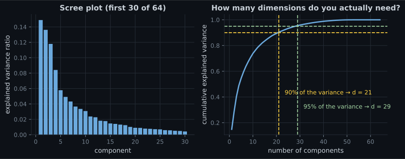
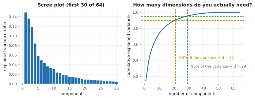
Choosing how many components

Fit PCA with all components, look at the cumulative explained variance, and cut where it flattens. On scikit-learn’s digits dataset — 1,797 images of $8 \times 8$ pixels, so 64 features:

The first component alone carries 14.89% and the second 13.62%.

figureScree plot and cumulative variancematplotlib

scikit-learn lets you state the target directly:

from sklearn.decomposition import PCA
 
pca = PCA(n_components=0.90, svd_solver="full").fit(X)   # a float means "this much variance"
print(pca.n_components_)          # 21

from sklearn.decomposition import PCA
 
pca = PCA(n_components=0.90, svd_solver="full").fit(X)   # a float means "this much variance"
print(pca.n_components_)          # 21

Do not use PCA output dimensionality as a hyperparameter tuned on the test set. If $d$ affects downstream accuracy, put PCA in a pipeline and tune it in cross-validation, exactly as with any other preprocessing step.

Standardise first, or PC1 becomes a unit conversion

This is the failure that actually happens in practice. The wine dataset has 13 chemical measurements whose raw standard deviations range from 0.12 (nonflavanoid_phenolsnonflavanoid_phenols) to 314.0 (prolineproline, measured in mg/L).

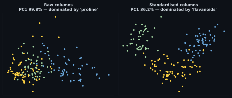
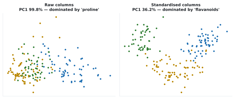
PC1 on the raw data explains 99.81% of the variance — and it is the proline column, at a loading of 0.9998. PCA has faithfully reported that one column has a bigger number in it than the others. That is a fact about milligrams per litre, not about wine.

After standardising, PC1 explains a modest 36.2% and mixes 13 features, with flavanoidsflavanoids leading at 0.4229. Much less impressive, and actually informative.

figureWine cultivars, before and after standardisingmatplotlib

Always:

from sklearn.decomposition import PCA
from sklearn.pipeline import make_pipeline
from sklearn.preprocessing import StandardScaler
 
pipe = make_pipeline(StandardScaler(), PCA(n_components=0.95))

from sklearn.decomposition import PCA
from sklearn.pipeline import make_pipeline
from sklearn.preprocessing import StandardScaler
 
pipe = make_pipeline(StandardScaler(), PCA(n_components=0.95))

The exception is data whose columns already share units and where relative magnitude is meaningful — pixel intensities, spectra, or a block of columns all in dollars.

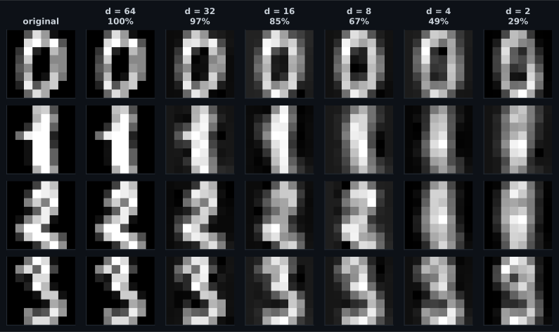
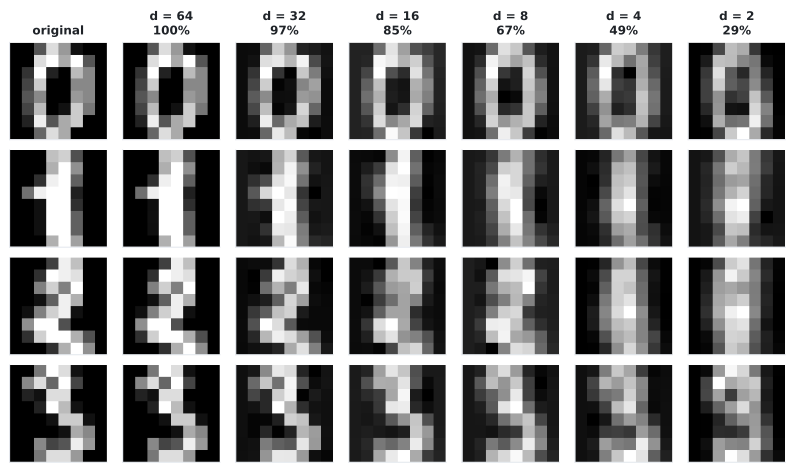
Reconstruction, compression and denoising

inverse_transforminverse_transform maps back to the original space. What comes out is the projection of the input onto the retained subspace — the closest possible approximation using $d$ directions.

figureThe same digits at six compression levelsmatplotlib

Halving the storage costs 3.4% of the variance. That is the compression trade in one row.

The same mechanism denoises. Noise is, by construction, spread evenly across all directions, while signal concentrates in the top few. Projecting to a low-dimensional subspace and back discards mostly noise:

import numpy as np
from sklearn.datasets import load_digits
from sklearn.decomposition import PCA
 
X = load_digits().data
rng = np.random.default_rng(0)
X_noisy = X + rng.normal(0, 4, X.shape)
 
pca = PCA(n_components=0.80, random_state=0).fit(X_noisy)
X_clean = pca.inverse_transform(pca.transform(X_noisy))
 
print("components kept", pca.n_components_)
print("MSE noisy vs original", round(float(((X_noisy - X) ** 2).mean()), 3))
print("MSE clean vs original", round(float(((X_clean - X) ** 2).mean()), 3))

import numpy as np
from sklearn.datasets import load_digits
from sklearn.decomposition import PCA
 
X = load_digits().data
rng = np.random.default_rng(0)
X_noisy = X + rng.normal(0, 4, X.shape)
 
pca = PCA(n_components=0.80, random_state=0).fit(X_noisy)
X_clean = pca.inverse_transform(pca.transform(X_noisy))
 
print("components kept", pca.n_components_)
print("MSE noisy vs original", round(float(((X_noisy - X) ** 2).mean()), 3))
print("MSE clean vs original", round(float(((X_clean - X) ** 2).mean()), 3))

In code

import numpy as np
from sklearn.decomposition import PCA
 
X = np.array([[2.0, 1.0], [3.0, 3.0], [4.0, 2.0], [5.0, 5.0], [6.0, 4.0]])
 
pca = PCA().fit(X)
 
print("mean_                 ", pca.mean_)                        # [4. 3.]
print("explained_variance_   ", pca.explained_variance_)          # [4.5 0.5]
print("explained_variance_ratio_", pca.explained_variance_ratio_) # [0.9 0.1]
print("components_ (rows are PCs)\n", pca.components_.round(4))
# [[ 0.7071  0.7071]
#  [-0.7071  0.7071]]
 
Z = pca.transform(X)
print("PC1 scores", Z[:, 0].round(4))    # [-2.8284 -0.7071 -0.7071  2.1213  2.1213]
 
# One component only, then back out again
p1 = PCA(n_components=1).fit(X)
X_rec = p1.inverse_transform(p1.transform(X))
print("total squared error", round(float(((X - X_rec) ** 2).sum()), 4))   # 2.0

import numpy as np
from sklearn.decomposition import PCA
 
X = np.array([[2.0, 1.0], [3.0, 3.0], [4.0, 2.0], [5.0, 5.0], [6.0, 4.0]])
 
pca = PCA().fit(X)
 
print("mean_                 ", pca.mean_)                        # [4. 3.]
print("explained_variance_   ", pca.explained_variance_)          # [4.5 0.5]
print("explained_variance_ratio_", pca.explained_variance_ratio_) # [0.9 0.1]
print("components_ (rows are PCs)\n", pca.components_.round(4))
# [[ 0.7071  0.7071]
#  [-0.7071  0.7071]]
 
Z = pca.transform(X)
print("PC1 scores", Z[:, 0].round(4))    # [-2.8284 -0.7071 -0.7071  2.1213  2.1213]
 
# One component only, then back out again
p1 = PCA(n_components=1).fit(X)
X_rec = p1.inverse_transform(p1.transform(X))
print("total squared error", round(float(((X - X_rec) ** 2).sum()), 4))   # 2.0

That last number is $(n-1)\lambda_2 = 4 \times 0.5 = 2.0$ — the discarded eigenvalue, recovered empirically.

Randomised and incremental PCA

svd_solver="randomized"svd_solver="randomized" approximates the top $d$ singular vectors with random projections, turning $O(n p^2)$ into roughly $O(n p d)$. It only pays when the matrix is large and $d \ll p$: on the $1797 \times 64$ digits matrix it was slower than the full SVD, while on a $5000 \times 800$ matrix asking for 50 components it was about twice as fast. scikit-learn’s svd_solver="auto"svd_solver="auto" picks sensibly, so leave it alone unless you have measured.

IncrementalPCAIncrementalPCA processes the data in batches and never holds it all in memory:

import numpy as np
from sklearn.decomposition import IncrementalPCA
 
ipca = IncrementalPCA(n_components=32, batch_size=256)
for batch in np.array_split(X, 20):        # or read from disk, one chunk at a time
    ipca.partial_fit(batch)
 
X_reduced = ipca.transform(X)

import numpy as np
from sklearn.decomposition import IncrementalPCA
 
ipca = IncrementalPCA(n_components=32, batch_size=256)
for batch in np.array_split(X, 20):        # or read from disk, one chunk at a time
    ipca.partial_fit(batch)
 
X_reduced = ipca.transform(X)

Use it when the data does not fit in RAM, or when it arrives as a stream.

Kernel PCA

PCA is a linear method: it can only find flat subspaces. If the structure is curved, no rotation will straighten it.

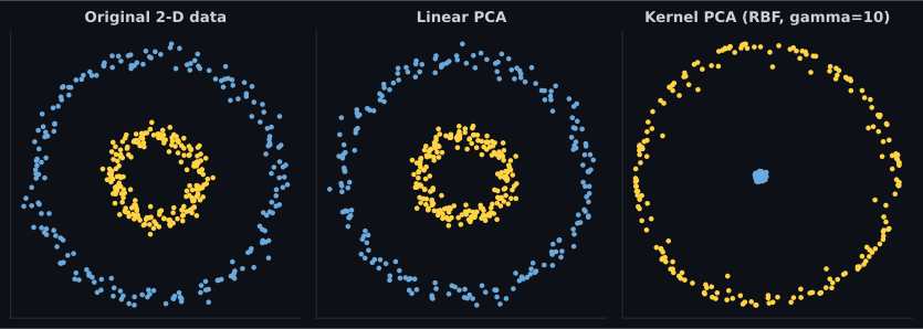
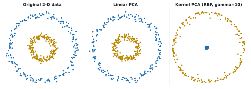
Kernel PCA applies the kernel trick — implicitly map to a high-dimensional space, do linear PCA there, and never form the mapping explicitly. On two concentric circles:

figureLinear PCA cannot unfold a circle; an RBF kernel canmatplotlib

Two costs. Kernel PCA is $O(n^2)$ in memory because it builds the kernel matrix, and inverse_transforminverse_transform requires fit_inverse_transform=Truefit_inverse_transform=True and is only approximate — the pre-image problem has no exact solution.

Pitfalls

Not standardising. Measured above: PC1 at 99.81% that is a single column’s units. This is the most common PCA mistake by a wide margin.

Fitting on the full dataset before splitting. PCA learns the components from the data, so fitting on train + test leaks test-set structure into the transform. Put it in a PipelinePipeline.

Assuming high variance means high relevance. PCA is unsupervised — it has never seen yy. A low-variance direction can be the one that predicts the target. If you need supervised dimension reduction, use linear discriminant analysis or partial least squares.

Interpreting components as features. PC1 is a weighted mixture of every original column. “PC1 increased by 2” is not a sentence anyone outside the model can act on.

Applying PCA to one-hot encoded categoricals. The variance of a one-hot column is $p(1-p)$, which is a fact about category frequency, not importance. Use multiple correspondence analysis or a learned embedding.

Expecting inverse_transforminverse_transform to be lossless. It returns the projection onto the retained subspace. With $d < p$ the discarded variance is gone permanently.

Reading meaning into a component’s sign. Eigenvectors are defined up to sign. A loading of $-0.42$ and $+0.42$ describe the same structure.

Reaching for svd_solver="randomized"svd_solver="randomized" without measuring. On the digits matrix it was slower than the exact solver. It wins on large, wide matrices — measure before switching.

Compare

🧪 Try It Yourself

Exercise 1 – Eigendecomposition by hand

Exercise 2 – Confirm against scikit-learn

Exercise 3 – The discarded eigenvalue is the error

Exercise 4 – Standardising changes everything

Exercise 5 – The compression curve

Recap

• PCA maximises projected variance, which is identical to minimising squared reconstruction error — Pythagoras on centred data.
• The Lagrangian gives $\mathbf{C}\mathbf{u} = \lambda\mathbf{u}$: components are eigenvectors and their variances are the eigenvalues.
• The five-point example gave $\lambda = 4.5, 0.5$, EVR 90%/10%, PC1 $= (0.7071, 0.7071)$, and a one-component reconstruction error of exactly $(n-1)\lambda_2 = 2.0$.
• scikit-learn uses the SVD, which is numerically better and avoids forming a $p \times p$ matrix.
• Digits needs 21 of 64 components for 90% of the variance, 29 for 95%.
• Standardise first. On raw wine data PC1 explains 99.81% and is the proline column’s units; standardised it explains 36.2% and separates the cultivars.
• inverse_transforminverse_transform is the projection, not the original: $d = 32$ costs 3.4% of the variance, $d = 2$ costs 71.5%.
• PCA is linear. Concentric circles stay inseparable at 0.4375 accuracy until an RBF kernel takes it to 0.6575.

Exercise 6 – Price each variance target in components

Next

t-SNE and Manifold Learning — what to do when the data lies on a curved manifold that no rotation can flatten, and why the prettiest plots in machine learning are also the easiest to over-read.