Learning Rate Scheduling

Decaying the learning rate is standard advice, and it is good advice — but the measurements below put a number on it, and that number is smaller than the enthusiasm suggests. Getting the base rate right matters far more than the shape of the curve you decay it along, which is why this page starts with the range test.

What you’ll learn

• The five standard schedules written as functions, with their values tabulated epoch by epoch.
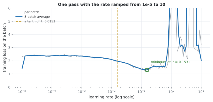
• The learning-rate range test: one pass, 120 batches, rate ramped from 1e-5 to 10, minimum loss at lr = 0.1531.
• Why the usual “take a tenth of the minimum” rule suggested 0.0153 when 0.1 worked better.
• Five schedules trained identically: constant 0.8510 against a best of 0.8525 — a gain of 0.0015.
• Where scheduling genuinely paid: ReduceLROnPlateau over 60 epochs reached 0.8690, cutting the rate seven times.
• How to implement any schedule three ways in Keras, and which to prefer.

Get the base rate right first

$$\theta \leftarrow \theta - \eta_t \nabla_\theta L$$

Everything on this page changes $\eta_t$ over time. None of it helps if $\eta_0$ is wrong: the gradient descent page measured a 1,000× too small rate producing 0.1320 accuracy — a schedule cannot rescue that.

The range test finds a good base rate in about one epoch of compute. Start absurdly low, multiply the rate by a constant factor every batch, and record the loss:

120 batches, rate from 1e-5 to 10

optimizer = keras.optimizers.SGD(1e-5)
for step in range(120):
    rate = 1e-5 * (10.0 / 1e-5) ** (step / 119)
    optimizer.learning_rate.assign(rate)
    # ... one gradient step on the next batch, record the loss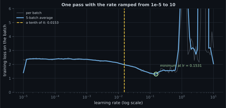

figure One pass with the rate ramped from 1e-5 to 10 matplotlib

Three regions. Below about 1e-3 nothing happens — the loss barely moves from its initial 2.4. Between 1e-3 and 0.15 the loss falls steadily. Past roughly 0.8 it diverges, exceeding the plot. The smoothed minimum sits at lr = 0.1531; the dashed line is the conventional tenth of that.

Learning rate	Loss on that batch
0.00001	2.3408
0.00065	2.3288
0.00263	2.1945
0.01060	2.0891
0.04268	1.7232
0.17191	1.3173
0.69237	1.4831
2.78855	3.2875
10.00000	3.2027

The smoothed minimum is at 0.1531, and the standard recipe is to train at roughly a tenth of it — 0.0153 — on the theory that the minimum is already at the edge of stability.

Here that recipe was too conservative. The schedule comparison below trains at a constant 0.1, close to the range test’s minimum rather than a tenth of it, and reaches 0.8510. The rule of thumb is a starting point for a sweep, not an answer: read the range test as “1e-3 is far too low and 0.8 diverges” and then try two or three rates in between.

The five schedules

diagram Diagram mermaid

  flowchart TD
  A["run the range test"] --> B["sweep two or three rates
inside the useful band"]
  B --> C{"does the run plateau
before the budget ends?"}
  C -- no --> D["a constant rate is fine
measured: 0.8510"]
  C -- yes --> E{"can you afford
extra epochs?"}
  E -- yes --> F["ReduceLROnPlateau
cuts only when progress stops"]
  E -- no --> G["1cycle or piecewise
needs the total step count"]
  H["never combine a schedule object
with ReduceLROnPlateau"] -.-> F

Each schedule is a function of the step count

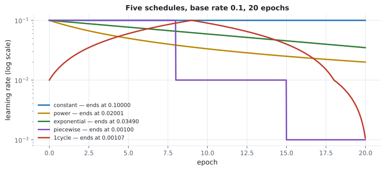
BASE, STEPS_PER_EPOCH, TOTAL = 0.1, 63, 1260
 
def constant(step):     return BASE
 
def power_decay(step):  return BASE / (1 + step / (STEPS_PER_EPOCH * 5))
 
def exponential(step):  return BASE * 0.9 ** (step / (STEPS_PER_EPOCH * 2))
 
def piecewise(step):
    epoch = step / STEPS_PER_EPOCH
    return BASE if epoch < 8 else BASE / 10 if epoch < 15 else BASE / 100
 
def one_cycle(step):
    """Ramp up to the peak over 45% of training, back down, then anneal."""
    peak, start = BASE, BASE / 10
    up, down = int(0.45 * TOTAL), int(0.9 * TOTAL)
    if step < up:    return start + (peak - start) * step / up
    if step < down:  return peak - (peak - start) * (step - up) / (down - up)
    return start * (1 - 0.9 * min((step - down) / max(TOTAL - down, 1), 1.0))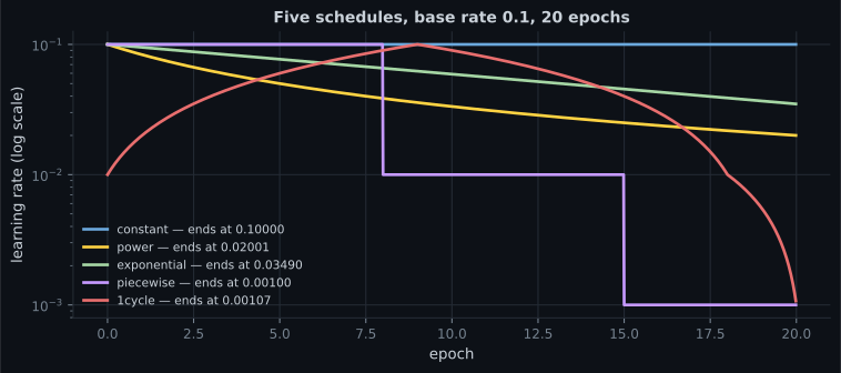

figure Five schedules, base rate 0.1, 20 epochs matplotlib

The shapes differ far more than the results will. Note that 1cycle starts an order of magnitude below the base rate and only reaches it at epoch 9 — the ramp-up is a deliberate warm-up, and the final anneal takes it below every other schedule.

Schedule	Epoch 0	Epoch 5	Epoch 10	Epoch 15	Epoch 19
constant	0.10000	0.10000	0.10000	0.10000	0.10000
power	0.10000	0.05000	0.03333	0.02500	0.02083
exponential	0.10000	0.07684	0.05905	0.04538	0.03675
piecewise	0.10000	0.10000	0.01000	0.00100	0.00100
1cycle	0.01000	0.06000	0.09000	0.04000	0.00550

What the schedules actually bought

Same architecture, same seed, same 20-epoch budget, same base rate, SGD, 8,000 Fashion-MNIST rows:

figure Five schedules, identical everything else matplotlib

The whole spread is 0.0045 — from power decay's 0.8480 to piecewise and 1cycle's 0.8525. Constant, the schedule that does nothing at all, scored 0.8510. On this budget with a well-chosen base rate, the schedule is not what decides the result.

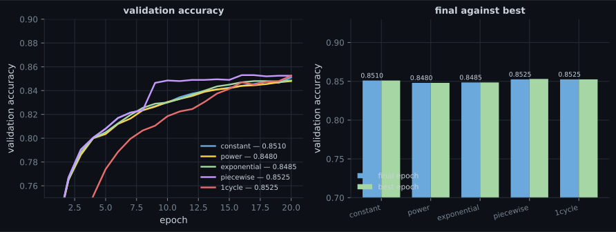
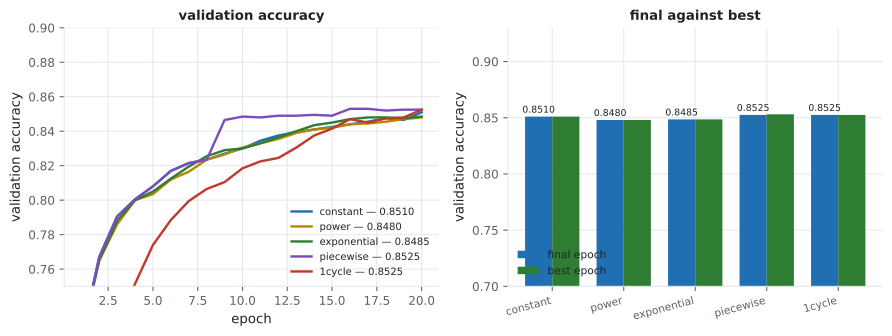
Schedule	Final val accuracy	Best val accuracy	Best epoch	Final training loss
constant	0.8510	0.8510	20	0.3514
power	0.8480	0.8480	20	0.4178
exponential	0.8485	0.8485	20	0.3782
piecewise	0.8525	0.8530	16	0.4090
1cycle	0.8525	0.8525	20	0.3939

The best schedule beat doing nothing by 0.0015. Two of the five were worse than constant. On a 2,000-row validation set that entire spread is inside the noise band, which means the honest summary is: at a well-chosen base rate on a short run, scheduling did not measurably help.

Notice also that constant reached the lowest training loss (0.3514) while finishing mid-table on validation. The decaying schedules trade training loss for a smoother approach — which is the mechanism they are supposed to provide, and here it was worth almost nothing.

Where it did pay

ReduceLROnPlateau watches the validation loss and cuts the rate when progress stops, so it schedules in response to the run rather than to a clock. Over 60 epochs at base rate 0.1:

Epoch it fired	New rate	Validation loss	Validation accuracy
34	0.050000	0.4233	0.8530
39	0.025000	0.4099	0.8620
43	0.012500	0.4016	0.8660
47	0.006250	0.3962	0.8675
51	0.003125	0.3942	0.8685
55	0.001563	0.3939	0.8690
58	0.000781	0.3943	0.8655

Seven reductions, and accuracy climbed from 0.8530 to 0.8690 — a gain of 0.0160, roughly ten times what any fixed schedule delivered.

Read that carefully, because there is a confound: this run had 60 epochs against the fixed schedules’ 20. Part of the gain is simply more training. What the table does show cleanly is the mechanism — every cut in the rate is followed by an immediate drop in validation loss, and the first cut only happened at epoch 34, which is long after any of the fixed schedules had already decayed most of the way down. A plateau schedule spends the high rate for as long as the high rate is still working. A clock-based schedule cannot know that.

sketch Compare schedule shapes p5.js Pause Restart

The five schedules drawn from the same formulas used in the measured runs. Click a schedule to isolate it, and drag the epoch marker to read the exact rate.

Three ways to write a schedule in Keras

1. A LearningRateSchedule object, passed to the optimizer

schedule = keras.optimizers.schedules.ExponentialDecay(
    initial_learning_rate=0.1, decay_steps=126, decay_rate=0.9)
model.compile(keras.optimizers.SGD(schedule), loss="...")

2. A callback that recomputes the rate every epoch

def by_epoch(epoch, rate):
    return 0.1 / (1 + epoch / 5)
 
model.fit(..., callbacks=[keras.callbacks.LearningRateScheduler(by_epoch)])

3. React to the metric instead of the clock

model.fit(..., callbacks=[keras.callbacks.ReduceLROnPlateau(
    monitor="val_loss", factor=0.5, patience=3, min_lr=1e-5)])

Form 1 is per-step and is the one to use for anything smooth — it is also what gets saved with the optimizer, so a reloaded model resumes on the right part of the curve. Form 2 is per-epoch, which is coarser but easier to reason about. Form 3 is the only one that adapts to what is actually happening.

Verified: ExponentialDecay(0.1, 126, 0.9) matches $0.1 \times 0.9^{\text{step}/126}$ to 7.13e-09 across steps 0 through 2,520.

sketch The measured table, ranked p5.js Pause Restart

Click a column to rank every row by it. The bars are that column's values and the highest and lowest are computed from the numbers, not written in.

Pitfalls

• Scheduling before tuning the base rate. The base rate is worth an order of magnitude; the schedule was worth 0.0015 here.
• Trusting the “one tenth of the range-test minimum” rule. It suggested 0.0153; 0.1 trained better. Use the test to bracket, then sweep.
• Comparing schedules on one seed. The entire spread across five schedules was 0.0045, well inside seed-to-seed noise on a 2,000-row validation set.
• Mixing a schedule object with ReduceLROnPlateau. The callback cannot override a LearningRateSchedule passed to the optimizer — it writes to a value the schedule ignores. Pick one mechanism.
• Decaying too early. The plateau schedule did not touch the rate until epoch 34, and every cut after that helped. A clock-based decay would have cut it at epoch 8.
• Forgetting that 1cycle starts low. Its first epochs run at a tenth of the base rate by design; a short run may never reach the peak.
• Assuming a schedule fixes divergence. If the base rate is past the stability limit, the early steps have already destroyed the weights.

Recap

• The range test found the loss minimum at lr 0.1531 and divergence past roughly 0.8, in one epoch of compute.
• The conventional tenth-of-the-minimum rule gave 0.0153, while 0.1 trained better — treat the test as a bracket.
• Five schedules on identical 20-epoch runs spanned 0.8480 to 0.8525, with constant at 0.8510. Two schedules were worse than no schedule.
• Constant reached the lowest training loss and mid-table validation accuracy; decay trades one for the other, and here the trade was worth almost nothing.
• ReduceLROnPlateau over 60 epochs cut the rate seven times and reached 0.8690, though it also had three times the epochs.
• Keras offers per-step schedule objects, per-epoch callbacks, and metric-driven reduction. Do not combine the first with the third.

Next

Six pages of individual techniques, and the question of how to assemble them into a process that works on a problem you have not seen before: The Universal Workflow of Machine Learning.

pch.quizTag pch.quizDefaultTitle

1. Five schedules on identical runs gave 0.8480 to 0.8525, with a constant rate at 0.8510. What is the correct conclusion?

   A Schedules are useless and should never be used B At a well-chosen base rate on a short run, the schedule's shape made no measurable difference here — the entire spread is within seed noise, so the base rate deserved the tuning effort instead C Piecewise decay is the best schedule D The experiment was too small to conclude anything
   pch.quizShowAnswer

   B — At a well-chosen base rate on a short run, the schedule's shape made no measurable difference here — the entire spread is within seed noise, so the base rate deserved the tuning effort instead — Two of the five were worse than doing nothing. That is the signature of a difference inside the noise band, not of a ranking.

2. The range test's minimum was at lr = 0.1531 and the usual rule suggests training at a tenth of that. What happened when the rate was set to 0.1 instead?

   A Training diverged B It trained well and reached 0.8510 — the tenth-of-the-minimum rule was too conservative here, so the test is best read as a bracket (1e-3 too low, 0.8 diverges) to sweep inside C It made no difference at all D The loss went to nan after one epoch
   pch.quizShowAnswer

   B — It trained well and reached 0.8510 — the tenth-of-the-minimum rule was too conservative here, so the test is best read as a bracket (1e-3 too low, 0.8 diverges) to sweep inside — The test tells you where the useful range is. Picking a single number from it by formula is less reliable than trying two or three rates inside the range.

3. Why can ReduceLROnPlateau outperform a clock-based decay?

   A Because it uses a smaller learning rate overall B Because it only reduces the rate when validation loss stops improving — in the measured run it left the rate at 0.1 until epoch 34, whereas a fixed schedule would have decayed it from epoch 8 C Because it also applies early stopping D Because it changes the rate every batch rather than every epoch
   pch.quizShowAnswer

   B — Because it only reduces the rate when validation loss stops improving — in the measured run it left the rate at 0.1 until epoch 34, whereas a fixed schedule would have decayed it from epoch 8 — Spending the high rate for as long as it is still working is the whole advantage. The confound in that run is that it also had three times the epochs.

4. What goes wrong if you pass a LearningRateSchedule object to the optimizer and also add ReduceLROnPlateau?

   A Keras raises an error immediately B The callback writes a value the schedule ignores, so the reduction silently has no effect — the schedule keeps computing the rate from the step count C The two rates are multiplied together D Training becomes much slower
   pch.quizShowAnswer

   B — The callback writes a value the schedule ignores, so the reduction silently has no effect — the schedule keeps computing the rate from the step count — Nothing errors, so it is easy to believe the reduction is working. Choose one mechanism: a schedule object, a callback, or plateau reduction.

5. 1cycle starts at a tenth of the base rate and reaches the peak at epoch 9 of 20. What does that imply for a short run?

   A It converges faster than everything else B A run shorter than the ramp-up never reaches the peak rate at all, so 1cycle's behaviour depends on knowing the total number of steps in advance C The base rate should be set ten times higher D It behaves identically to exponential decay
   pch.quizShowAnswer

   B — A run shorter than the ramp-up never reaches the peak rate at all, so 1cycle's behaviour depends on knowing the total number of steps in advance — Every 1cycle implementation takes the total step count as a parameter for exactly this reason. Change the epoch count and you change the schedule.

🧪 Try It Yourself

pch.exerciseTag pch.exerciseTitle

pch.exerciseTag pch.exerciseTitle

pch.exerciseTag pch.exerciseTitle

pch.exerciseTag pch.exerciseTitle

pch.exerciseTag pch.exerciseTitle

pch.exerciseTag pch.exerciseTitle