What you’ll learn

• the five rule metrics — support, confidence, lift, leverage and conviction — each derived and each computed by hand on the same baskets
• why confidence alone is dangerous, shown with a rule at 80% confidence and lift 1.23
• a rule with lift 0.31: buying chips makes bread less likely
• the downward-closure property, and the candidate counts it eliminates: 70 → 0 at level 4
• the full Apriori loop traced level by level on 20 baskets
• why the number of rules explodes, and how to control it
• FP-Growth, and when the level-wise scan stops being viable

Intuition

Every technique so far in this phase has grouped rows. Association rule learning groups columns — or rather, it finds columns that tend to be present together.

The classic setting is a supermarket. Each transaction is a set of items. You want statements like “customers who buy bread also buy butter” — and, much more importantly, you want to know which of those statements are worth acting on.

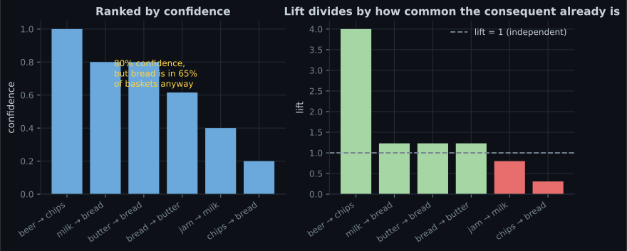
That second part is where almost all the difficulty lives. “Customers who buy anchovies also buy bread” is true 80% of the time. It is also useless, because 65% of all customers buy bread. The rule tells you nothing you did not already know from the shelf.

Distinguishing a real association from a popular consequent is the whole job, and it requires more than one number.

  flowchart LR
  T["Transactions
(sets of items)"] --> F["Frequent itemsets
support >= min_support"]
  F --> R["Candidate rules
split each itemset into A -> B"]
  R --> M["Score each rule:
confidence, lift, leverage, conviction"]
  M --> K["Keep the rules that beat
independence, not just the popular ones"]

The data

Twenty baskets, small enough to count by hand:

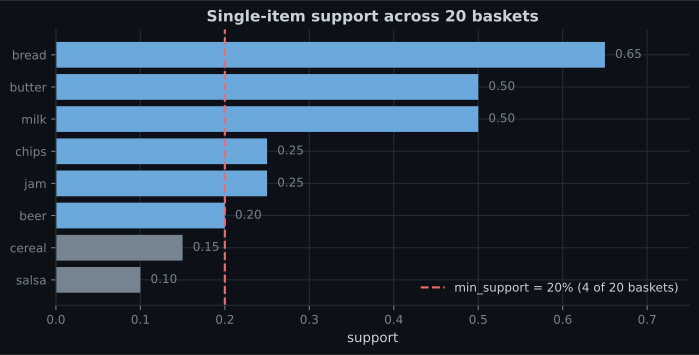
Item counts, which are the foundation of everything below:

figureLevel 1 of Apriori: count every itemmatplotlib

The math

Write $T$ for the set of transactions, $|T| = N$, and $\sigma(X)$ for the number of transactions containing itemset $X$.

Support — how often the itemset appears at all:

Confidence of the rule $A \Rightarrow B$ — the conditional probability:

Lift — confidence divided by the consequent’s base rate:

This is the ratio of the observed joint frequency to the frequency expected under independence. Read it as:

• $\text{lift} > 1$ — $A$ and $B$ appear together more often than chance. Positive association.
• $\text{lift} = 1$ — independent. The rule tells you nothing.
• $\text{lift} < 1$ — they appear together less often than chance. Negative association.

Lift is symmetric: $\operatorname{lift}(A \Rightarrow B) = \operatorname{lift}(B \Rightarrow A)$. Confidence is not.

Leverage — the same comparison as a difference rather than a ratio:

Zero under independence. Because it is a difference, it weights by how many transactions are actually affected — useful when a huge lift comes from a handful of baskets.

Conviction — how much more often the rule would be wrong if $A$ and $B$ were independent:

It is 1 under independence and $\infty$ when confidence is 1 (the rule has no counterexamples). Unlike lift, conviction is directional.

Worked example by hand

bread ⇒ butter

Bread appears in 13 baskets, butter in 10, and both together in 8 (baskets 1, 2, 5, 9, 11, 15, 17, 20).

A mild positive association: butter is about 23% more likely in a bread basket than in a random one.

The same pair, reversed

The confidence jumped from 0.62 to 0.80 while the lift did not move at all. Confidence went up purely because bread is more common than butter — swapping the direction changed the denominator, not the relationship. Lift, being symmetric, is unfooled.

Conviction does change: $(1 - 0.65)/(1 - 0.80) = 0.35/0.20 = 1.7500$ against 1.3000 the other way. It is directional by design, and it says the butter ⇒ bread direction is the stronger prediction.

beer ⇒ chips

Beer appears in 4 baskets (6, 8, 12, 19), chips in 5 (6, 8, 12, 16, 19). Together: 4.

Every beer basket contains chips. Lift 4.0 means four times the chance expected by independence, and conviction is infinite because there is not a single counterexample.

chips ⇒ bread, the rule that is worse than nothing

Chips appears in 5 baskets, bread in 13, both together in 1 (basket 19).

Lift 0.31. Chips buyers are three times less likely to buy bread than a random customer. Negative leverage confirms it. That is a real, actionable finding — the two are substitutes, not complements — and it is invisible to anyone who only ranks by confidence.

The full table

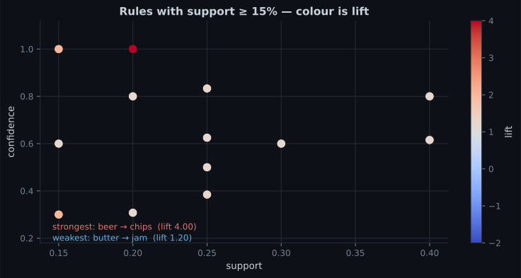
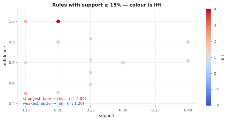
Four rules sit at exactly 0.8000 confidence, and their lifts range from 4.00 down to 1.23. Ranking by confidence would put chips ⇒ beerchips ⇒ beer — a genuinely strong rule — level with three bread-is-popular truisms.

figureConfidence and lift tell different storiesmatplotlib

figureEvery rule as a pointmatplotlib

The Apriori algorithm

Naively, finding all frequent itemsets over $m$ items means checking $2^m - 1$ subsets. With just 100 products that is more than $10^{30}$ candidates.

Apriori’s insight is the downward-closure property (also called the Apriori property):

Adding an item to an itemset can only reduce the number of baskets containing it. So:

If an itemset is infrequent, every superset of it is infrequent.

That contrapositive lets you prune whole branches without counting them. The algorithm becomes a level-wise scan:

1. Count all 1-itemsets; keep those with support $\ge$ min_supportmin_support. Call this $L_1$.
2. Generate candidate $(k{+}1)$-itemsets by joining pairs in $L_k$ that share $k-1$ items.
3. Prune any candidate having a $k$-subset that is not in $L_k$ — no counting needed.
4. Scan the transactions once to count the survivors; keep the frequent ones as $L_{k+1}$.
5. Stop when $L_{k+1}$ is empty.

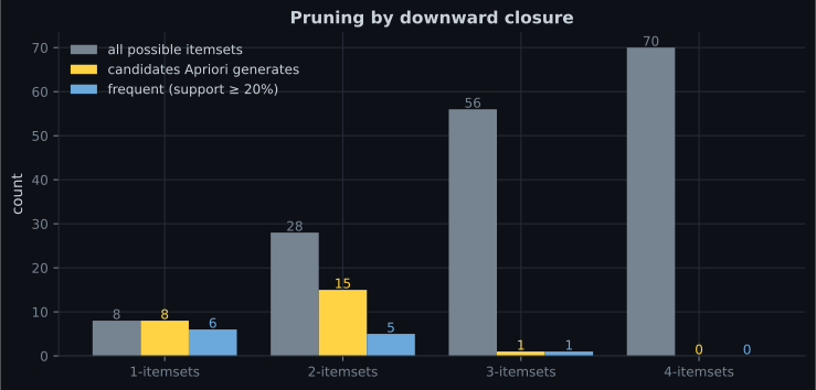
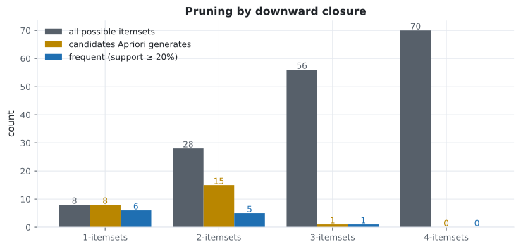
Traced on the twenty baskets

With min_support = 0.20min_support = 0.20:

At level 1, cereal (0.15) and salsa (0.10) drop out. At level 2, Apriori only builds candidates from the 6 survivors — 15 pairs rather than 28 — and 5 clear the threshold. At level 3 only one candidate survives pruning, {bread, butter, milk}{bread, butter, milk} at support 0.25. At level 4 there is nothing left to join, so the algorithm stops after examining 24 candidates instead of 162.

figureDownward closure collapses the searchmatplotlib

From itemsets to rules

Each frequent itemset of size $k$ yields $2^k - 2$ candidate rules — every way of splitting it into a non-empty antecedent and a non-empty consequent. For {bread, butter, milk}{bread, butter, milk} at support 0.25, that is 6 rules:

Note the support is 0.25 for all six — it is a property of the itemset, not of how you split it. Only the confidence and lift differ.

  flowchart LR
  I["Frequent itemset
{bread, butter, milk}
support 0.25"] --> R1["bread, butter -> milk"]
  I --> R2["butter, milk -> bread"]
  I --> R3["bread -> butter, milk"]
  R1 --> S1["conf 0.625
lift 1.250"]
  R2 --> S2["conf 0.833
lift 1.282"]
  R3 --> S3["conf 0.385
lift 1.282"]

See it move

Item D has support 0.12, below the threshold. The moment it goes red, every itemset containing it — AD, BD, CD, ABD, ACD, BCD, ABCD, seven of the fifteen nodes — is pruned without a single count.

The next sketch is the metrics themselves: move the overlap between two item sets and watch confidence and lift disagree.

Click to swap the base rates. With $\operatorname{supp}(B) = 0.65$, confidence can reach 0.8 while lift is barely above 1. Drop $B$ to 0.25 and the same overlap produces a far higher lift — because the same co-occurrence is now genuinely surprising.

In code

scikit-learn does not implement Apriori. The standard library is mlxtendmlxtend:

pip install mlxtend

pip install mlxtend

import pandas as pd
from mlxtend.frequent_patterns import apriori, association_rules
from mlxtend.preprocessing import TransactionEncoder
 
baskets = [
    ["bread", "butter", "milk"], ["bread", "butter"], ["bread", "milk", "jam"],
    ["butter", "milk"], ["bread", "butter", "milk", "jam"], ["beer", "chips"],
    ["bread", "jam"], ["beer", "chips", "salsa"], ["bread", "butter", "jam"],
    ["milk", "cereal"], ["bread", "butter", "milk"], ["beer", "chips"],
    ["bread", "milk"], ["butter", "jam"], ["bread", "butter", "milk", "cereal"],
    ["chips", "salsa"], ["bread", "butter"], ["milk", "cereal", "bread"],
    ["beer", "chips", "bread"], ["bread", "butter", "milk"],
]
 
# One-hot: one row per basket, one boolean column per item.
te = TransactionEncoder()
df = pd.DataFrame(te.fit_transform(baskets), columns=te.columns_)
 
freq = apriori(df, min_support=0.20, use_colnames=True)
print(freq.sort_values("support", ascending=False))
 
rules = association_rules(freq, metric="lift", min_threshold=1.0)
cols = ["antecedents", "consequents", "support", "confidence", "lift", "leverage", "conviction"]
print(rules[cols].sort_values("lift", ascending=False).round(4))

import pandas as pd
from mlxtend.frequent_patterns import apriori, association_rules
from mlxtend.preprocessing import TransactionEncoder
 
baskets = [
    ["bread", "butter", "milk"], ["bread", "butter"], ["bread", "milk", "jam"],
    ["butter", "milk"], ["bread", "butter", "milk", "jam"], ["beer", "chips"],
    ["bread", "jam"], ["beer", "chips", "salsa"], ["bread", "butter", "jam"],
    ["milk", "cereal"], ["bread", "butter", "milk"], ["beer", "chips"],
    ["bread", "milk"], ["butter", "jam"], ["bread", "butter", "milk", "cereal"],
    ["chips", "salsa"], ["bread", "butter"], ["milk", "cereal", "bread"],
    ["beer", "chips", "bread"], ["bread", "butter", "milk"],
]
 
# One-hot: one row per basket, one boolean column per item.
te = TransactionEncoder()
df = pd.DataFrame(te.fit_transform(baskets), columns=te.columns_)
 
freq = apriori(df, min_support=0.20, use_colnames=True)
print(freq.sort_values("support", ascending=False))
 
rules = association_rules(freq, metric="lift", min_threshold=1.0)
cols = ["antecedents", "consequents", "support", "confidence", "lift", "leverage", "conviction"]
print(rules[cols].sort_values("lift", ascending=False).round(4))

Doing it without a dependency is about fifteen lines, and worth writing once:

from itertools import combinations
 
def support(itemset, baskets):
    s = set(itemset)
    return sum(1 for b in baskets if s <= set(b)) / len(baskets)
 
def apriori(baskets, min_support):
    """Level-wise search with downward-closure pruning."""
    items = sorted({i for b in baskets for i in b})
    frequent = {frozenset([i]) for i in items if support([i], baskets) >= min_support}
    all_frequent, prev, k = dict(), frequent, 2
 
    while prev:
        for fs in prev:
            all_frequent[fs] = support(fs, baskets)
        candidates = set()
        for a, b in combinations(prev, 2):
            union = a | b
            if len(union) != k:
                continue
            # PRUNE: every k-1 subset must already be frequent
            if all(frozenset(s) in prev for s in combinations(union, k - 1)):
                candidates.add(union)
        prev = {c for c in candidates if support(c, baskets) >= min_support}
        k += 1
    return all_frequent
 
freq = apriori(baskets, 0.20)
for fs, s in sorted(freq.items(), key=lambda kv: (-kv[1], sorted(kv[0]))):
    print(f"{s:.2f}  {set(sorted(fs))}")

from itertools import combinations
 
def support(itemset, baskets):
    s = set(itemset)
    return sum(1 for b in baskets if s <= set(b)) / len(baskets)
 
def apriori(baskets, min_support):
    """Level-wise search with downward-closure pruning."""
    items = sorted({i for b in baskets for i in b})
    frequent = {frozenset([i]) for i in items if support([i], baskets) >= min_support}
    all_frequent, prev, k = dict(), frequent, 2
 
    while prev:
        for fs in prev:
            all_frequent[fs] = support(fs, baskets)
        candidates = set()
        for a, b in combinations(prev, 2):
            union = a | b
            if len(union) != k:
                continue
            # PRUNE: every k-1 subset must already be frequent
            if all(frozenset(s) in prev for s in combinations(union, k - 1)):
                candidates.add(union)
        prev = {c for c in candidates if support(c, baskets) >= min_support}
        k += 1
    return all_frequent
 
freq = apriori(baskets, 0.20)
for fs, s in sorted(freq.items(), key=lambda kv: (-kv[1], sorted(kv[0]))):
    print(f"{s:.2f}  {set(sorted(fs))}")

Controlling the explosion

Rule counts grow ferociously as you loosen min_supportmin_support. Three defences:

Set min_supportmin_support from a count, not a fraction. “At least 50 baskets” is a statement you can defend; “0.001” is not. Compute the fraction from the count you need.

Filter on lift and leverage. Lift alone promotes rules built on three transactions. Leverage weights by how many baskets are actually affected, so requiring both lift > 1.2lift > 1.2 and leverage > 0.01leverage > 0.01 removes the noise.

Restrict the consequent. If you only care about what drives one product, ask only for rules with that item on the right:

target = {"butter"}
useful = rules[
    (rules["consequents"] == frozenset(target))
    & (rules["lift"] > 1.2)
    & (rules["leverage"] > 0.01)
].sort_values("lift", ascending=False)

target = {"butter"}
useful = rules[
    (rules["consequents"] == frozenset(target))
    & (rules["lift"] > 1.2)
    & (rules["leverage"] > 0.01)
].sort_values("lift", ascending=False)

FP-Growth

Apriori scans the whole transaction database once per level. On millions of transactions with tens of thousands of items, that is the bottleneck.

FP-Growth builds a compressed prefix tree (the FP-tree) in two passes and then mines it recursively without generating candidates at all. It is typically an order of magnitude faster and gives identical results — the frequent itemsets are a property of the data, not of the algorithm.

from mlxtend.frequent_patterns import fpgrowth
 
freq_fp = fpgrowth(df, min_support=0.20, use_colnames=True)
# Same itemsets, same supports, different route.

from mlxtend.frequent_patterns import fpgrowth
 
freq_fp = fpgrowth(df, min_support=0.20, use_colnames=True)
# Same itemsets, same supports, different route.

Use Apriori to learn the concepts and for small data. Use FP-Growth in production.

Pitfalls

Ranking by confidence. Four rules on this page share confidence 0.8000 with lifts from 1.23 to 4.00. Confidence rewards popular consequents; sort by lift or leverage.

Ignoring lift below 1. chips ⇒ breadchips ⇒ bread at lift 0.31 is one of the most informative rules in the set — the items are substitutes. Most tooling filters these out by default with min_threshold=1.0min_threshold=1.0.

Reading causation into co-occurrence. Beer and chips co-occur; neither causes the other. Both are caused by the same occasion. Acting on the rule (place them together) can still be correct; explaining it as causation is not.

Setting min_supportmin_support too low. The candidate count grows super-exponentially. Below about 0.01 on a real retail dataset you will exhaust memory before the level-3 scan finishes.

Forgetting the base rates. Every metric on this page is relative to $\operatorname{supp}(B)$. An item in 90% of baskets can never produce an interesting rule, because confidence cannot exceed 1 and the lift ceiling is $1/0.9 = 1.11$.

Trusting rules built on a handful of transactions. A rule with support 0.001 and lift 12 rests on maybe five baskets. Check the raw count, and use leverage, which is bounded by how much of the data is affected.

Treating the item vocabulary as fixed. “Milk” and “semi-skimmed milk 2L” are different items to the algorithm. Aggregating to a sensible product hierarchy before mining usually matters more than any parameter.

Compare

🧪 Try It Yourself

Exercise 1 – Support by counting

Exercise 2 – Confidence is not symmetric, lift is

Exercise 3 – Find the negative association

Exercise 4 – Downward closure in action

Exercise 5 – All five metrics at once

Recap

• Support counts how often; confidence is $\hat{P}(B \mid A)$; lift compares that against independence.
• Confidence is directional, lift is symmetric: bread ⇒ butter and butter ⇒ bread gave 0.6154 and 0.8000 confidence but the same 1.2308 lift.
• Four different rules in the data share confidence 0.8000 with lifts from 1.23 to 4.00. Never rank by confidence alone.
• chips ⇒ breadchips ⇒ bread has lift 0.3077 and leverage -0.1125 — a real negative association that a lift > 1lift > 1 filter would discard.
• Leverage demotes high-lift rules resting on a handful of baskets; conviction is infinite when a rule has no counterexamples.
• Downward closure — an infrequent itemset has no frequent supersets — pruned the search from 162 possible itemsets to 24 ever counted.
• Apriori scans the database once per level; FP-Growth does it in two passes and returns identical results.

Exercise 6 – Confidence without lift is a trap

Next

Principal Component Analysis (PCA) — the second half of this phase. Instead of grouping rows or items, PCA reduces the number of columns, and it does it by finding the directions along which the data actually varies.