First Example: Classifying Movie Reviews (IMDB, Binary)

Positive review or negative review. Two classes, 25,000 labelled examples, and a model small enough to train on a laptop in seconds — which makes this the right place to build the habits that matter: measure a baseline before you build, watch validation and training separately, and treat the decision threshold as a knob rather than a constant.

What you’ll learn

• What the raw data actually is — integer sequences, median length 178, and the off-by-three index shift that silently corrupts every decode.
• Why multi-hot encoding turns 25,000 reviews into a 1 GB matrix that is 98.7% zeros, and what it throws away.
• The two baselines to beat: majority class 0.5000 and logistic regression 0.8618 on the same features.
• Binary cross-entropy computed by hand to a difference of 0.00e+00 against Keras.
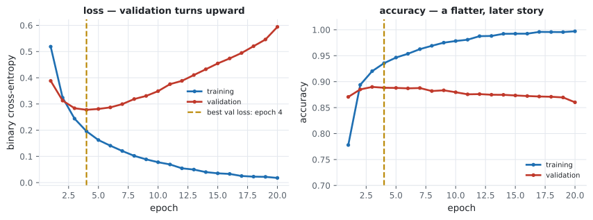
• The exact epoch where validation loss turns: epoch 4 at 0.2777, rising to 0.5941 by epoch 20 while training loss falls to 0.0178.
• Why dropout bought only 0.0034 of validation loss here, and L2 made the best epoch worse.
• Why the 0.5 threshold cost accuracy: 0.8792 at 0.50 against 0.8855 at 0.65.

The data is not text

imdb.load_data hands you lists of integers, not strings. Each integer is a word’s frequency rank in the corpus, and num_words=10000 keeps only the 10,000 most common ranks.

The raw shape of the problem

from tensorflow import keras
 
(raw_train, y_train), (raw_test, y_test) = keras.datasets.imdb.load_data(
    num_words=10000)
 
print(len(raw_train), len(raw_test))              # 25000 25000
print(y_train[:5])                                # [1 0 0 1 0]
print(max(max(review) for review in raw_train))   # 9999
print(float(y_train.mean()))                      # 0.5 -- exactly balanced

Measured over the 25,000 training reviews:

	Tokens
shortest review	11
median	178
mean	238.7
99th percentile	926
longest	2,494

figure What 25,000 reviews look like before any model sees them matplotlib

The mean sits well above the median because the tail is long: half the reviews are under 178 tokens, but the longest is 2,494. On the right, each row is one review's multi-hot vector. Only 1.32% of the matrix is ones overall, and just 0.32% past index 2,000 — indices are frequency ranks, so the common-word end of the vocabulary is where almost every review lands.

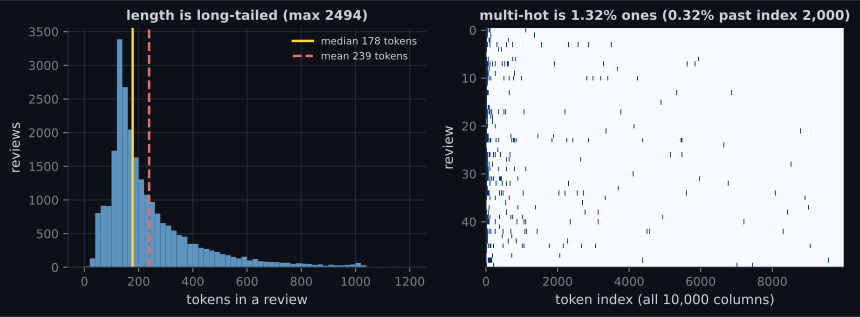
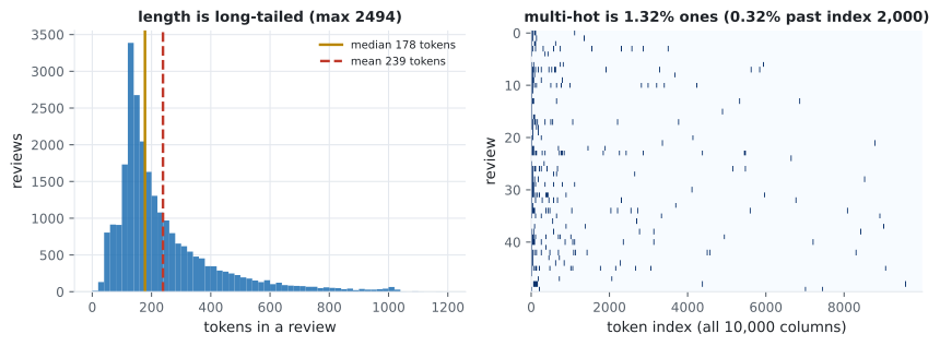
The class balance is exactly 0.5, which is unusual and convenient: accuracy is a meaningful score here in a way it will not be on the Reuters page, where one topic holds 35% of the data.

The index shift that ruins every decode

The word index maps words to ranks starting at 1, but indices 0, 1 and 2 are reserved inside the sequences for padding, start-of-sequence and unknown-word. So the sequence integer for a word is its rank plus 3:

Decoding, correctly

index = keras.datasets.imdb.get_word_index()
reverse = {value + 3: key for key, value in index.items()}
reverse.update({0: "<pad>", 1: "<start>", 2: "<unk>", 3: "<unused>"})
 
print(" ".join(reverse.get(token, "?") for token in raw_train[0][:10]))
# <start> this film was just brilliant casting location scenery story

Drop the + 3 and the decode still produces fluent-looking English — every word shifted three ranks along. Nothing crashes and the output looks plausible, which is exactly the class of bug worth knowing about in advance.

Multi-hot encoding

A Dense layer needs a fixed-width numeric vector, and reviews have variable length. The simplest fix is to ignore order entirely: one column per vocabulary word, 1 if the word appears anywhere in the review.

diagram Diagram mermaid

  flowchart LR
  A["raw review
variable length text"] --> B["integer sequence
ranks, offset by 3"]
  B --> C["multi-hot vector
10,000 columns, 1 if present"]
  C --> D["Dense 16 relu"]
  D --> E["Dense 16 relu"]
  E --> F["Dense 1 sigmoid
P(positive)"]

One column per vocabulary word

import numpy as np
 
def multi_hot(sequences, dimension=10000):
    out = np.zeros((len(sequences), dimension), dtype="float32")
    for i, sequence in enumerate(sequences):
        out[i, sequence] = 1.0
    return out
 
x_train = multi_hot(raw_train)
print(x_train.shape, f"{x_train.nbytes:,} bytes")
# (25000, 10000) 1,000,000,000 bytes
print(float(x_train.mean()))   # 0.013174 -- 1.32% ones

That is a 1 GB array holding 1.32% ones, and the test set costs another gigabyte. It works at this scale and stops working immediately past it, which is the entire motivation for the embedding layers of Phase 4.

Multi-hot also discards two things:

• Order. “not good at all” and “good, not at all bad” encode identically when they share a word set.
• Repetition. [1, 3, 3, 7] and [1, 3, 7] produce the same vector — the row is a set membership test, not a count.

sketch Build a multi-hot vector by hand p5.js Pause Restart

Click vocabulary cells to append tokens to a review. The vector below fills in with ones. Click a token you already used and nothing changes: multi-hot records presence, not count.

Baselines before the network

Two numbers, both cheap, both worth having before you write a single layer:

Baseline	Test accuracy
always predict the majority class	0.5000
logistic regression on the same features (5,000 rows)	0.8531
logistic regression on the same features (all 25,000)	0.8618

A linear model on the same input reaches 0.8618. If the network lands at 0.86 it has learned nothing a single matrix multiply could not. This is the bar, and skipping it is how a project ends up celebrating a network that underperforms LogisticRegression.

The model

Three layers, one output

model = keras.Sequential([
    keras.layers.Input((10000,)),
    keras.layers.Dense(16, activation="relu"),
    keras.layers.Dense(16, activation="relu"),
    keras.layers.Dense(1, activation="sigmoid"),
])
model.compile("rmsprop", "binary_crossentropy", metrics=["accuracy"])

The parameter count is worth reading:

Layer	Parameters
Dense(16) on 10,000 inputs	$10{,}000 \times 16 + 16 = 160{,}016$
Dense(16) on 16 inputs	$16 \times 16 + 16 = 272$
Dense(1) on 16 inputs	$16 \times 1 + 1 = 17$
total	160,305

99.8% of the parameters sit in the first layer, purely because the input is 10,000 wide. Widening the hidden layers barely moves the total; widening the vocabulary moves it linearly.

Sigmoid and binary cross-entropy

One output unit with a sigmoid produces $\hat{y} \in (0, 1)$, read as $P(\text{positive})$. The matching loss is binary cross-entropy:

$$L = -\frac{1}{N} \sum_{i=1}^{N} \Big[ y_i \log \hat{y}_i + (1 - y_i) \log (1 - \hat{y}_i) \Big]$$

Only one term survives per row: if $y_i = 1$ the loss is $-\log \hat{y}_i$, and if $y_i = 0$ it is $-\log(1 - \hat{y}_i)$. Both are the negative log of the probability the model assigned to the correct answer. Worked by hand on four predictions:

$\hat{y}$	$y$	$-\log$ (probability of the truth)
0.90	1	0.105361
0.20	0	0.223144
0.60	1	0.510826
0.05	1	2.995732

Mean: 0.958766. Keras returns 0.958766 — a difference of 0.00e+00.

Notice the distribution of blame. Three of the four predictions contribute 0.839 between them; the single confident-and-wrong prediction contributes 2.996, which is 78% of the total from 25% of the rows. That asymmetry is the point of a log loss: nearly indifferent to mild errors, brutal about confident ones. Accuracy would have scored that row as one mistake out of four.

Where it starts overfitting

Train on 15,000 rows, validate on the held-out 10,000:

Twenty epochs, watching both curves

history = model.fit(x_train[:15000], y_train[:15000], epochs=20,
                    batch_size=512,
                    validation_data=(x_train[15000:], y_train[15000:]))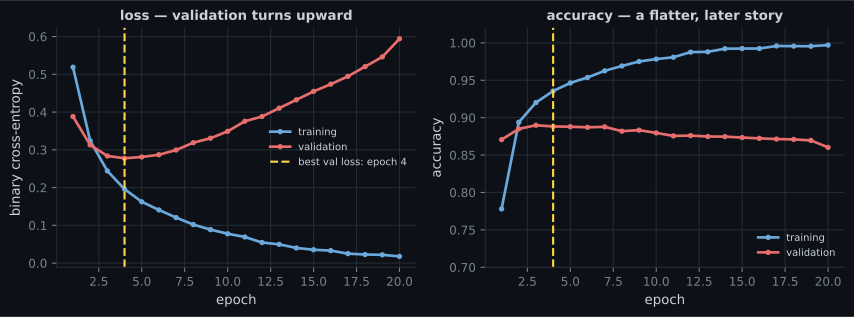

figure Twenty epochs, and only the first four helped matplotlib

Validation loss reaches 0.2777 at epoch 4 and is 2.14x worse by epoch 20. Training loss keeps falling to 0.0178 the whole time — the model is still improving on data it has already seen. Validation accuracy tells a much softer version of the same story, drifting from 0.8898 down to 0.8602 while the loss more than doubles.

Epoch	Training loss	Validation loss	Validation accuracy
1	0.5188	0.3882	0.8706
2	0.3240	0.3129	0.8850
3	0.2441	0.2837	0.8898
4	0.1959	0.2777	0.8882
5	0.1623	0.2811	0.8879
10	0.0778	0.3490	0.8796
15	0.0354	0.4547	0.8734
20	0.0178	0.5941	0.8602

Read the two validation columns against each other. Loss doubles between epoch 4 and epoch 20; accuracy falls by 0.028. Loss is the sensitive instrument. It sees the model becoming more confident about its errors — the same effect the hand-worked table showed, where one confident mistake outweighed three near-misses. Accuracy cannot see confidence at all: a prediction of 0.51 and one of 0.99 count identically.

Also worth noting: the best validation accuracy (0.8898) arrives at epoch 3, one epoch before the best validation loss. The two metrics do not agree on when to stop, and neither is wrong — they are answering different questions.

Retrain at the epoch that was best

Once you know the number, train from scratch on all 25,000 rows for exactly that many epochs:

One fresh model, four epochs, one evaluation

final = build_model()          # fresh weights, not the trained model
final.fit(x_train, y_train, epochs=4, batch_size=512)
print(final.evaluate(x_test, y_test))
# test loss 0.3081, test accuracy 0.8792

0.8792 on the test set, against logistic regression’s 0.8618 on the same features. The network is worth about 1.7 accuracy points here — not the order of magnitude the phrase “deep learning” suggests. On a bag-of-words representation, most of the available signal genuinely is linear.

Note also that 0.8792 is lower than the 0.8882 validation accuracy at epoch 4. That is the expected direction: the epoch was chosen by looking at the validation set, so that score is optimistic. The test set is the one number you have not spent.

Does regularisation help?

figure Dropout and L2 against the plain network matplotlib

Dropout 0.5 reached 0.2743 at epoch 6 — 0.0034 better than the plain model's best, and two epochs later. L2 = 0.001 was worse at its best (0.3282) but far more stable: by epoch 20 it sat at 0.4429 against the plain model's 0.5941.

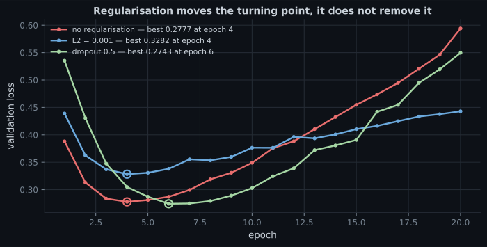
Variant	Best validation loss	At epoch	Val accuracy there	Val loss at epoch 20
none	0.2777	4	0.8882	0.5941
L2 = 0.001	0.3282	4	0.8881	0.4429
dropout 0.5	0.2743	6	0.8916	0.5495

The honest reading is less flattering than the usual one. Dropout bought 0.0034 of validation loss and 0.0034 of accuracy — real, reproducible, and tiny. L2 made the best epoch worse, by 0.05. What both actually did was flatten the penalty for training too long: at epoch 20 the L2 model is 0.15 ahead of the plain one.

So on this problem regularisation is insurance against overtraining rather than a source of accuracy. If you already stop at the best epoch, you have collected most of what it offers. That balance shifts as models grow relative to their data — a theme Phase 2 develops properly.

The threshold is a choice

model.predict returns probabilities. Turning those into labels requires a cutoff, and 0.5 is a default, not an answer:

Threshold	Accuracy	Precision	Recall
0.20	0.8234	0.7469	0.9782
0.35	0.8601	0.8011	0.9581
0.50	0.8792	0.8436	0.9310
0.65	0.8855	0.8801	0.8926
0.80	0.8741	0.9147	0.8251

Moving the cutoff from 0.50 to 0.65 gains 0.0063 accuracy for free — no retraining, no new data. The model’s probabilities are slightly optimistic about the positive class, and shifting the threshold corrects for it. (Choose that cutoff on validation data, not on the test set, or you have simply moved the selection bias somewhere less visible.)

The wider point is that accuracy is one row of this table. When a false positive and a false negative cost different amounts, pick the threshold that reflects the difference and report precision and recall instead of a single number.

sketch One trained model, five thresholds p5.js Pause Restart

Drag the handle across the five measured thresholds. Accuracy, precision and recall are the trained IMDB model's real test-set numbers at each cutoff.

Pitfalls

• Forgetting the + 3 index shift when decoding. Nothing errors; every word is simply wrong by three frequency ranks.
• Reporting the best epoch’s validation score as your result. You selected that epoch using the validation set, so it is optimistic. The test number here is 0.8792, not 0.8882.
• Skipping the baseline. Logistic regression gets 0.8618 on these exact features. Without that number, 0.8792 sounds like a triumph.
• Reading accuracy instead of loss for overfitting. Between epoch 4 and 20, accuracy fell 0.028 while loss doubled. Accuracy is blind to confidence.
• Multi-hot at 1 GB per 25,000 rows. The cost is vocabulary times rows, regardless of how long the reviews are. Embeddings exist for this reason.
• Assuming 0.5 is the threshold. It cost 0.0063 accuracy here, and the right cutoff depends on which error is more expensive.
• Treating a balanced dataset as normal. IMDB is exactly 50/50 by construction. Reuters is not, and accuracy stops being informative there.

Recap

• The dataset is integer sequences with a median length of 178, exactly balanced between classes, and the sequence-to-word mapping is offset by 3.
• Multi-hot gives a fixed-width input at the cost of order, repetition, and 1 GB of mostly-zero memory.
• The baselines are 0.5000 (majority) and 0.8618 (logistic regression). Both must be beaten before a network is worth anything.
• Sigmoid plus binary cross-entropy is the standard binary pairing; the loss is the negative log-probability of the truth, verified to 0.00e+00 by hand.
• Validation loss bottoms out at epoch 4 (0.2777) and more than doubles by epoch 20 while training loss keeps falling. Retrain at that epoch and evaluate once: 0.8792.
• Dropout gained 0.0034 and L2 lost 0.05 at their best epochs; both mainly reduced the cost of training too long.
• Sweeping the decision threshold gained more accuracy (0.0063) than either regulariser.

Next

The same pipeline with 46 classes instead of 2 changes the output layer, the loss function, and — most importantly — whether accuracy means anything at all: Classifying Newswires (Reuters).

pch.quizTag pch.quizDefaultTitle

1. Between epoch 4 and epoch 20, validation accuracy fell from 0.8882 to 0.8602 while validation loss rose from 0.2777 to 0.5941. Why did the loss move so much more?

   A Loss and accuracy are computed on different data B Cross-entropy measures the probability assigned to the correct label, so growing confidence in wrong answers is punished heavily, while accuracy only counts which side of the threshold each prediction lands on C Accuracy is a noisier metric than loss D The learning rate changed during training
   pch.quizShowAnswer

   B — Cross-entropy measures the probability assigned to the correct label, so growing confidence in wrong answers is punished heavily, while accuracy only counts which side of the threshold each prediction lands on — One confident mistake at 0.05 contributes 2.996 to the loss — more than three mild errors combined. Accuracy scores it as a single miss.

2. Why is 0.8882 (validation accuracy at the best epoch) the wrong number to report as the model's performance?

   A It is measured on too few examples B The epoch was chosen by looking at the validation set, so that score is optimistically biased; the untouched test set gives 0.8792 C Validation accuracy is always higher than test accuracy D It should be averaged with the training accuracy
   pch.quizShowAnswer

   B — The epoch was chosen by looking at the validation set, so that score is optimistically biased; the untouched test set gives 0.8792 — Every decision made by looking at a split contaminates it, and choosing the epoch is a decision.

3. The multi-hot matrix for 25,000 reviews is 1 GB and 98.7% zeros. What does that tell you about scaling this approach?

   A Nothing — memory is cheap B Memory grows with vocabulary size times row count regardless of how many words a review actually contains, so a larger vocabulary or corpus becomes impractical and dense embeddings are needed C The model will overfit because of the zeros D Sparse matrices would make the network more accurate
   pch.quizShowAnswer

   B — Memory grows with vocabulary size times row count regardless of how many words a review actually contains, so a larger vocabulary or corpus becomes impractical and dense embeddings are needed — The cost is set by vocabulary x rows, not by content. An embedding layer stores one dense vector per token instead.

4. Logistic regression on the same multi-hot features reaches 0.8618; the network reaches 0.8792. What is the right conclusion?

   A The network is not worth using B Most of the signal in a bag-of-words representation is linear, so the network adds a modest 1.7 points — and the baseline is what makes that judgement possible at all C The baseline must have been computed incorrectly D Accuracy is the wrong metric for this comparison
   pch.quizShowAnswer

   B — Most of the signal in a bag-of-words representation is linear, so the network adds a modest 1.7 points — and the baseline is what makes that judgement possible at all — The gain is real but small. Without the baseline you would have no way to know whether 0.8792 was good.

5. Moving the decision threshold from 0.50 to 0.65 raised accuracy from 0.8792 to 0.8855 without retraining. Why is that possible?

   A The model's weights changed B The threshold does not affect what the model learned — it only converts probabilities to labels, and this model's probabilities were slightly biased toward the positive class C 0.65 is the mathematically optimal threshold for sigmoid outputs D The test set was reshuffled
   pch.quizShowAnswer

   B — The threshold does not affect what the model learned — it only converts probabilities to labels, and this model's probabilities were slightly biased toward the positive class — The threshold is a post-hoc decision rule. Choose it on validation data, guided by the relative cost of each error type.

🧪 Try It Yourself

pch.exerciseTag pch.exerciseTitle

pch.exerciseTag pch.exerciseTitle

pch.exerciseTag pch.exerciseTitle

pch.exerciseTag pch.exerciseTitle

pch.exerciseTag pch.exerciseTitle

pch.exerciseTag pch.exerciseTitle