
The Power of Ensembles - Why Combine Models?
What you’ll learn
Section titled “What you’ll learn”- Condorcet’s jury theorem: why 51% voters become an 84% committee
- the variance formula for an average, and the correlation term that caps the gain
- why diversity, not individual quality, is what an ensemble is buying
- a measured case where an ensemble beats none of its members, and why
- the three families — bagging, boosting, stacking — mapped onto the bias-variance decomposition
- what ensembles cost: interpretability, latency, and training time
Intuition
Section titled “Intuition”Ask one competent person a hard question and you get one answer, right about 60% of the time. Ask 101 of them and take the majority: 97.9%.
The arithmetic works only under a condition that is easy to state and hard to satisfy: the voters must be wrong in different ways. A hundred and one people who all read the same wrong textbook give you one wrong answer, a hundred and one times.
That single condition explains everything in this phase. Bagging manufactures diversity by resampling the data; random forests add feature randomness on top; boosting manufactures it by making each model specialise in the previous one’s failures; stacking gets it free by using different model families.
  flowchart TD
  A["Many models"] --> B{"Are their errors
uncorrelated?"}
  B -->|yes| C["Averaging cancels them
ensemble beats the members"]
  B -->|no| D["Averaging reproduces them
ensemble equals the members"]
  C --> E["The work is in manufacturing
disagreement"]
  D --> E
The math
Section titled “The math”Condorcet’s jury theorem
Section titled “Condorcet’s jury theorem”With independent voters each correct with probability , the majority is correct with probability
If this tends to 1 as grows. If it tends to zero — a committee of below-chance voters is more reliably wrong than any one of them.
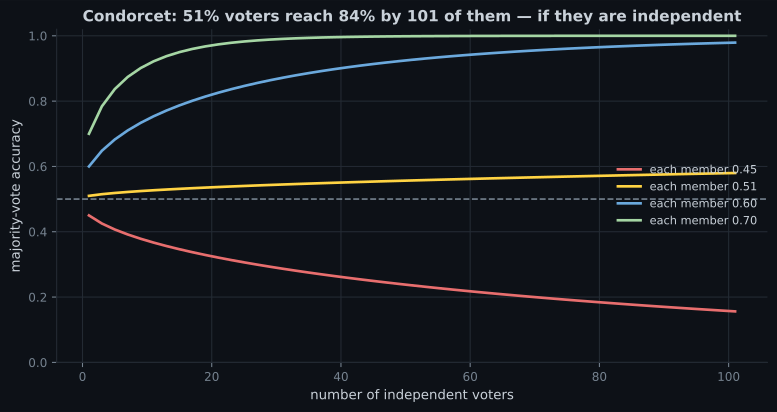
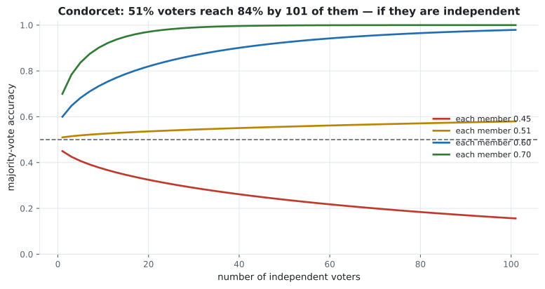
| Member accuracy | 1 voter | 11 | 51 | 101 |
|---|---|---|---|---|
| 0.45 | 0.450 | 0.367 | 0.236 | 0.156 |
| 0.51 | 0.510 | 0.527 | 0.557 | 0.580 |
| 0.60 | 0.600 | 0.754 | 0.927 | 0.979 |
| 0.70 | 0.700 | 0.922 | 0.999 | 1.000 |
The 0.51 row is the sober one. Barely-better-than-chance voters improve very slowly — 101 of them reach only 0.580. The theorem guarantees improvement; it says nothing about the rate.
The correlation term
Section titled “The correlation term”For models each with variance and average pairwise correlation , the variance of their average is
Two terms, and only one of them shrinks. As the second vanishes and you are left with
Correlation is a hard floor. No number of models gets you below it.
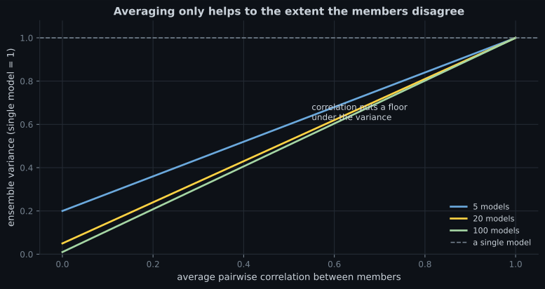
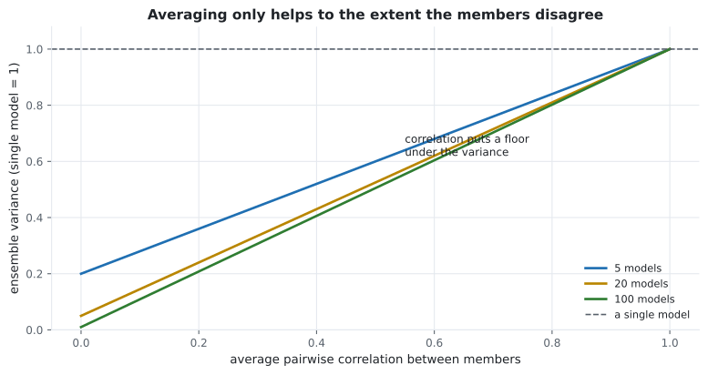
| 10 models | 100 models | Gain from 10 → 100 | |
|---|---|---|---|
| 0.0 | 0.100 | 0.010 | 10× |
| 0.3 | 0.370 | 0.307 | 1.2× |
| 0.6 | 0.640 | 0.604 | 1.06× |
| 0.9 | 0.910 | 0.901 | 1.01× |
This is the formula that justifies every design decision in the rest of the phase. A random forest samples features at each split as well as rows, purely to push down. Extra-Trees randomises the split thresholds too, accepting slightly worse individual trees for a lower — and usually wins.
Worked example by hand
Section titled “Worked example by hand”Three classifiers on five test rows. ✓ is correct, ✗ is wrong.
| Row | Model A | Model B | Model C | Majority | Correct? |
|---|---|---|---|---|---|
| 1 | ✓ | ✓ | ✗ | 2–1 correct | ✓ |
| 2 | ✓ | ✗ | ✓ | 2–1 correct | ✓ |
| 3 | ✗ | ✓ | ✓ | 2–1 correct | ✓ |
| 4 | ✓ | ✓ | ✓ | 3–0 correct | ✓ |
| 5 | ✗ | ✗ | ✗ | 3–0 wrong | ✗ |
| Accuracy | 0.6 | 0.6 | 0.6 | 0.8 |
Step 1 — the members. Each is right 3 times out of 5: 0.60.
Step 2 — the vote. Right on rows 1–4: 0.80.
Step 3 — where the gain came from. Rows 1, 2 and 3 each have exactly one model failing, and a different model each time. The majority survives every one.
Step 4 — where it did not. Row 5 has all three failing together. No vote can rescue that, and no fourth model of the same kind would either.
Step 5 — the counterfactual. Suppose all three models failed on rows 4 and 5 together instead — still 0.60 each, but now perfectly correlated. The majority scores 0.60. Identical member accuracy, no gain whatsoever. The 0.80 came from the pattern of the errors, not their count.
Diversity in pictures
Section titled “Diversity in pictures”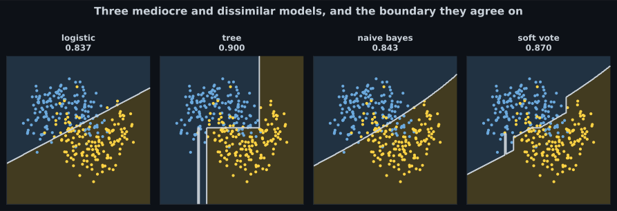
Reading the plot
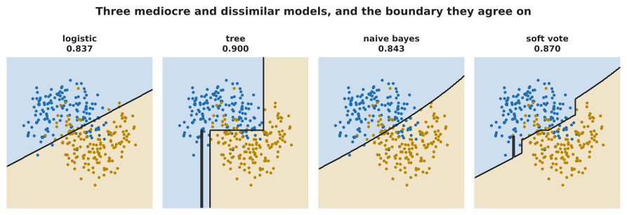
Section titled “Reading the plot”- Each member has a distinctive failure mode. Straight, rectangular, quadratic. Those are different shapes of wrongness, which is the useful kind of diversity.
- The vote’s boundary is not any of theirs. It follows the crescents better than the line and more smoothly than the staircase.
- Diversity here is free. No resampling and no reweighting — the model families disagree by construction. That is what makes voting and stacking the cheapest ensemble to build.
When an ensemble does not help
Section titled “When an ensemble does not help”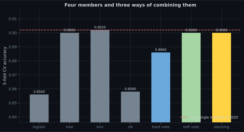
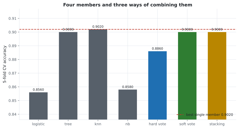
Measured on the same data with the same folds:
| Model | 5-fold CV accuracy |
|---|---|
| logistic regression | 0.8560 |
| decision tree (depth 4) | 0.9000 |
| KNN (k=15) | 0.9020 |
| Gaussian naive Bayes | 0.8580 |
| hard vote of all four | 0.8860 |
| soft vote of all four | 0.9000 |
| stacking with a logistic blender | 0.9000 |
No ensemble beat the best individual member. This is a real result on real folds, and it is here because the alternative — only showing the cases where ensembles win — would teach the wrong lesson.
What went wrong: two of the four members (logistic at 0.856 and naive Bayes at 0.858) are substantially weaker than KNN, and hard voting gives every member an equal say. Two weak votes can outvote one strong one. Soft voting recovers some of it by weighting by confidence, and stacking could learn to ignore the weak members — with 500 rows it does not have enough data to.
See it move
Section titled “See it move”Nine voters, each 60% accurate, deciding one question after another. The tally on the right is the committee’s running accuracy against the individual average.
The three families
Section titled “The three families”| Family | Members are | Built | Attacks | Example |
|---|---|---|---|---|
| Bagging | Strong, low bias, high variance | In parallel, on bootstrap samples | Variance | Random Forest |
| Boosting | Weak, high bias, low variance | Sequentially, each fixing the last | Bias | AdaBoost, XGBoost |
| Stacking | Whatever you have, ideally diverse | In parallel, then a blender learns the weights | Both | StackingClassifier |
Each maps directly onto a term of the bias-variance decomposition. Bagging averages away variance and leaves bias alone. Boosting drives bias down and slowly raises variance. Stacking learns a weighting that can improve either.
What ensembles cost
Section titled “What ensembles cost”| Cost | Detail |
|---|---|
| Interpretability | One tree is a set of rules; 300 trees is not |
| Prediction latency | Every member runs on every request |
| Training time | Roughly linear in members; boosting cannot be parallelised across them |
| Memory | The whole ensemble must be held and shipped |
| Debuggability | “Why this prediction?” needs SHAP rather than reading the model |
A single decision tree that scores 0.92 may be worth more than a forest at 0.94 if a regulator has to approve it.
Pitfalls
Section titled “Pitfalls”-
A committee of 101 voters, each 45% accurate, votes by majority. How accurate is the committee?
Condorcet's theorem cuts both ways. Below 50% per member, the majority converges toward zero: 101 below-chance voters are reliably wrong.
pch.quizShowAnswer
B — About 15.6% — worse than any individual — Condorcet's theorem cuts both ways. Below 50% per member, the majority converges toward zero: 101 below-chance voters are reliably wrong.
-
Your 100 models have average pairwise correlation 0.6. Roughly what fraction of a single model's variance remains?
Variance is rho + (1-rho)/n = 0.6 + 0.004 = 0.604. Correlation is a floor: 5 models would have reached 0.64, so the other 95 bought almost nothing.
pch.quizShowAnswer
C — 60% — Variance is rho + (1-rho)/n = 0.6 + 0.004 = 0.604. Correlation is a floor: 5 models would have reached 0.64, so the other 95 bought almost nothing.
-
Three models each score 0.60 and their vote scores 0.80. What produced the gain?
Had all three failed on the same two rows, the vote would also score 0.60. The gain came from the pattern of errors, not their count.
pch.quizShowAnswer
B — They failed on different rows, so a majority survived each individual failure — Had all three failed on the same two rows, the vote would also score 0.60. The gain came from the pattern of errors, not their count.
-
On the moons data, hard voting scored 0.8860 while its best member scored 0.9020. What is the most likely cause?
Hard voting gives every member an identical say. Logistic regression at 0.856 and naive Bayes at 0.858 can jointly outvote KNN at 0.902.
pch.quizShowAnswer
B — Two of the four members are markedly weaker, and equal votes let them outvote the strongest — Hard voting gives every member an identical say. Logistic regression at 0.856 and naive Bayes at 0.858 can jointly outvote KNN at 0.902.
🧪 Try It Yourself
Section titled “🧪 Try It Yourself”Exercise 1 – Condorcet by hand
Section titled “Exercise 1 – Condorcet by hand”Exercise 2 – The correlation floor
Section titled “Exercise 2 – The correlation floor”Exercise 3 – The five-row vote
Section titled “Exercise 3 – The five-row vote”Exercise 4 – Correlated members gain nothing
Section titled “Exercise 4 – Correlated members gain nothing”Exercise 5 – Check whether the ensemble actually wins
Section titled “Exercise 5 – Check whether the ensemble actually wins”- Condorcet: independent voters above 50% converge to certainty; below 50% they converge to certainty about the wrong answer.
- The variance of an average is . Correlation is a floor no ensemble size can breach.
- Three 0.60 models voting to 0.80 do so because they fail on different rows. Make them fail together and the vote scores 0.60.
- Measured counterexample: on the moons data, no combination of four members beat the best member. Hard voting actually lost 1.6 points.
- Bagging attacks variance, boosting attacks bias, stacking learns a weighting over both.
- The cost is interpretability, latency and training time, and it is sometimes not worth paying.
Exercise 6 – When does a majority vote help?
Section titled “Exercise 6 – When does a majority vote help?”Continue to Bagging - Random Forest Regressor/Classifier — manufacturing diversity by resampling, and getting a validation score for free while doing it.
pch.coffeeTagline
pch.coffeeCtapch.feedbackHeading
pch.feedbackSubheading