Phase 2 - Training Deep Neural Networks

Phase 1’s networks were two or three layers deep, because deeper ones do not train without help. This phase is that help: what breaks with depth, what fixes it, and — measured on identical runs — how much each fix is actually worth. Several are worth much less than their reputation, and one of them is routinely mis-measured because Keras reports a number that is not what it appears to be.

What this phase covers

diagram Diagram mermaid

  flowchart LR
  A["411 Backprop
and optimizers"] --> B["411.5 Loss functions
what to minimise"]
  B --> C["412 Vanishing and
exploding gradients"]
  C --> D["413 Batch
normalisation"]
  D --> E["414 Regularisation
and dropout"]
  E --> F["415 Learning rate
scheduling"]
  F --> G["416 The universal
workflow"]
  G --> H["417 Evaluating
models"]
  H --> I["418 Callbacks and
TensorBoard"]
  I --> J["Phase 3:
convolutional networks"]

Pages 411 to 415 are individual mechanisms. Pages 416 to 418 are the process that assembles them — which order to apply them in, how to know whether a number is real, and how to run the job.

The nine pages, and what each one proves

#	Page	The result it delivers
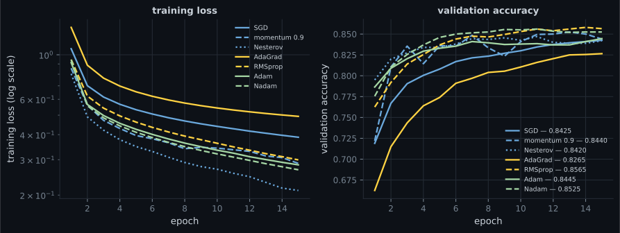
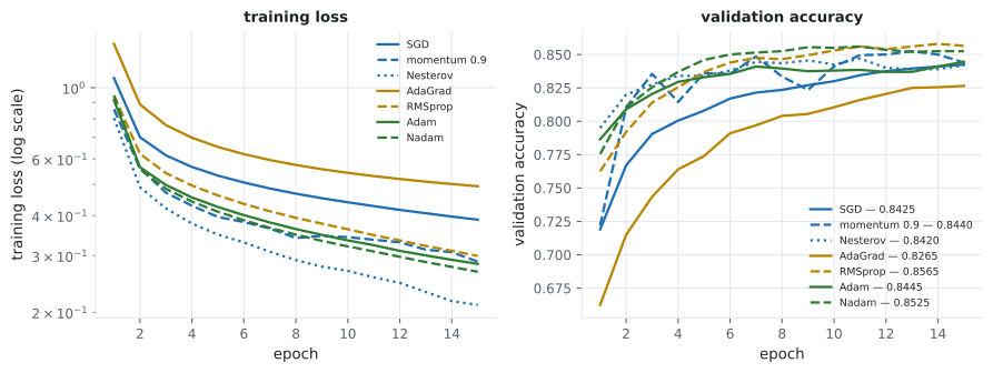
411	Backpropagation and Optimizers	Backprop matched to TensorFlow at 7.45e−09, and seven optimizers where RMSprop (0.8565) beat Adam (0.8445) while AdaGrad never arrived
411.5	Loss Functions	from_logits=False on a confident error returns a loss of 16.118095 instead of 40.0 with a gradient of exactly zero
412	Vanishing & Exploding Gradients	A 20-layer sigmoid network delivering 1.19e−12 to its first layer, and an exploding run that killed 127 of 128 units
413	Batch Normalization	Ten sigmoid layers going from 0.1025 to 0.9225 — and BN losing at batch size 4
414	Regularization & Dropout	Dropout 0.5 at 0.8633, and L2’s apparent ranking inverting once Keras’ penalty-inflated val_loss is corrected
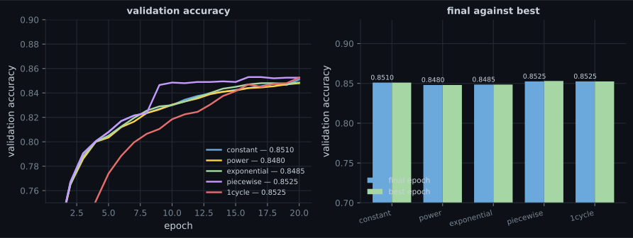
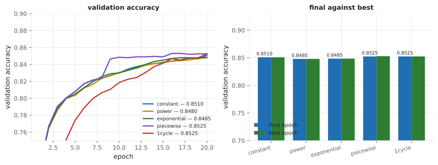
415	Learning Rate Scheduling	Five schedules within 0.0045 of each other, two of them worse than a constant rate
416	The Universal Workflow	A five-rung ladder from 0.1015 to 0.8635 where logistic regression alone covered 0.7385 of the climb
417	Evaluating Models	Thirty hold-out splits spanning 0.1417, and a leak reaching 0.9600 accuracy on pure noise
418	Callbacks and TensorBoard	Four policies, and proof that logs["loss"] mid-epoch is a running average, not the batch’s loss

figure Seven optimizers, one architecture, one seed matplotlib

Blue is the SGD family, amber the accumulating methods, green the Adam family. In the accuracy panel every optimizer except AdaGrad finishes inside a 0.014 band — but they arrive at very different times. Nesterov reaches the lowest training loss (0.2108) while finishing joint-lowest on validation accuracy, which is overfitting, not superiority.

figure Five schedules, identical everything else matplotlib

The whole spread is 0.0045 — from power decay's 0.8480 to piecewise and 1cycle's 0.8525. Constant, the schedule that does nothing at all, scored 0.8510. On this budget with a well-chosen base rate, the schedule is not what decides the result.

figure Every claim this phase set out to test matplotlib

Collected from the runs behind each page's own figures rather than measured afresh, so every bar is traceable to the page it names. Bar length is the log of the effect size, because the effects span from 0.0014 to 5,376 — the number that matters is printed on each bar. 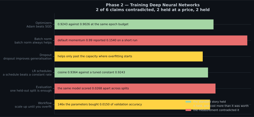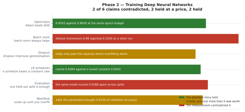Across all nine phases, 34 of 54 claims were contradicted outright, 11 held at a cost that was worth stating, and 9 held as advertised.

Five results that contradict the standard advice

1. Adam did not win. RMSprop finished 0.0120 ahead of it and Nadam 0.0080 ahead on the same problem. Adam beat plain SGD by 0.0020 — a difference no one should act on. What adaptive methods actually bought was time: 5 epochs to reach 0.84 against SGD’s 14. (411)
2. Learning-rate schedules bought almost nothing. Five schedules spanned 0.8480 to 0.8525 with a constant rate at 0.8510 — two schedules were worse than doing nothing. Getting the base rate right is worth an order of magnitude more. (415)
3. Batch normalisation did not raise the ceiling. At a well-tuned learning rate, with and without BN were identical to four decimal places (0.9115 both). BN’s value is tolerance: at lr=1.0 it scored 0.9380 against 0.3985. And at batch size 4 it lost. (413)
4. Keras’ val_loss inverted L2’s ranking. On the reported number every penalty looked worse than none; on the plain cross-entropy the strongest penalty was best by a wide margin (0.4810 against 0.6253). The reported loss includes the penalty term. (414)
5. A leak reached 0.9600 accuracy on data with no signal in it. Duplicating rows before a shuffled split let 1-nearest-neighbour find each test row’s twin in the training fold. Feature selection before the split scored 0.7550 where chance was 0.5100. (417)

The pattern across all five: the mechanisms are real, and their magnitudes are smaller and more conditional than the advice implies. The ones that mattered most here were the unglamorous ones — a correct base learning rate, a correct from_logits, an honest split.

What actually made the biggest difference

Ranked by measured effect on the same kind of problem:

Change	Measured effect
fixing a dead network (initialisation + clipping)	0.1025 → 0.8225
adding BN to ten stacked sigmoid layers	0.1025 → 0.9225
using from_logits=True on confident errors	a zero gradient becomes a usable one
beating a linear baseline at all	0.1015 → 0.8400
dropout 0.5 on an over-parameterised model	0.8467 → 0.8633
plateau-based rate reduction over 60 epochs	0.8530 → 0.8690
choosing RMSprop over Adam	0.8445 → 0.8565
the best fixed schedule over a constant rate	0.8510 → 0.8525

The top of that table is about making training work at all; the bottom is 0.001-level tuning. Most of the value is at the top, and most of the internet’s attention is at the bottom.

sketch The learning rate, on one axis p5.js Pause Restart

Drag through the sweep. Each stop is a measured run - the useful range is narrow and both edges fail in different ways.

sketch How often the standard story survived p5.js Pause Restart

Step through the phases. Each bar splits the claims that phase tested into contradicted, held at a price, and held as advertised - the totals are summed live.

Prerequisites

• Phase 1: tensors, the training loop, activations, and one gradient-descent step derived by hand.
• Comfort reading a training curve and telling training loss from validation loss.
• pip install tensorflow numpy matplotlib scikit-learn — no GPU needed. The heaviest measurement on any page in this phase is a 60-epoch run on 8,000 rows.

By the end of this phase you can

• Derive backpropagation for a small network and check it against GradientTape.
• Choose a loss from the target’s type, and explain why the sigmoid/cross-entropy pairing exists at all.
• Diagnose a dead or vanishing network from per-layer gradient norms rather than from the loss curve.
• Pick an initialiser that matches the activation, and know when clipping is a fix against a symptom.
• Insert normalisation where it helps and avoid it where it hurts.
• Regularise in the right order: capacity, then dropout, then a penalty.
• Find a base learning rate with a range test, and decide whether a schedule is worth adding.
• Build a baseline ladder and refuse to add complexity that does not pay.
• Design a validation scheme that does not leak, and report a spread rather than a point.
• Assemble a training job out of callbacks, and know exactly what each number it prints means.

Next

Everything so far treats an input as a flat vector. Images are not flat, and exploiting that structure is what Phase 3 is about: convolutional networks, where the architecture encodes the fact that nearby pixels are related.

pch.quizTag pch.quizDefaultTitle

1. Across this phase, which change produced the largest measured improvement?

   A Switching optimiser from SGD to Adam B Making a broken network train at all — initialisation and clipping took a dead run from 0.1025 to 0.8225, and BN took ten stacked sigmoid layers from 0.1025 to 0.9225 C Adding a learning-rate schedule D Increasing the model width
   pch.quizShowAnswer

   B — Making a broken network train at all — initialisation and clipping took a dead run from 0.1025 to 0.8225, and BN took ten stacked sigmoid layers from 0.1025 to 0.9225 — The large wins are about training working at all. The optimiser and schedule comparisons moved results by 0.001 to 0.01.

2. Five learning-rate schedules landed within 0.0045 of each other, with two worse than a constant rate. What is the takeaway?

   A Schedules are broken in Keras B The base rate deserves the tuning effort; the schedule's shape is a second-order effect on a short run at a well-chosen base rate C Only 1cycle is worth using D The measurement needs more epochs to be valid
   pch.quizShowAnswer

   B — The base rate deserves the tuning effort; the schedule's shape is a second-order effect on a short run at a well-chosen base rate — The same phase measured a 1,000x-too-small base rate producing 0.1320 accuracy. That is the difference worth chasing.

3. Why can Keras' reported val_loss not be used to compare L2 penalty strengths?

   A Because validation data is shuffled differently each epoch B Because the reported loss includes the regularisation term, so a stronger penalty inflates its own loss — comparing the raw numbers compares different quantities and inverted the true ranking here C Because L2 is applied only during training D Because val_loss is computed before the last update
   pch.quizShowAnswer

   B — Because the reported loss includes the regularisation term, so a stronger penalty inflates its own loss — comparing the raw numbers compares different quantities and inverted the true ranking here — Measured: 0.6469 versus 0.6253 on Keras' number, but 0.4810 versus 0.6253 on the plain cross-entropy.

4. Which order does the workflow page recommend for building a model?

   A Start with the largest model you can afford, then shrink it B Beat a dumb baseline, then build something that visibly overfits, then regularise it back — because a model with no generalisation gap has nothing to trade C Regularise first so the model never overfits D Tune hyperparameters before choosing an architecture
   pch.quizShowAnswer

   B — Beat a dumb baseline, then build something that visibly overfits, then regularise it back — because a model with no generalisation gap has nothing to trade — The measured 8-unit model had a gap of only 0.0221 and could not be improved by any regulariser: it was underfitting, and a small gap is only good news when the scores are high.

5. A colleague reports 0.86 validation accuracy from one 80/20 split on 600 rows. What should you ask for?

   A A larger model B A cross-validated mean with its spread — thirty random splits of the same 600 rows ranged from 0.7333 to 0.8750, so a single split cannot support a comparison C The training accuracy D A different random seed
   pch.quizShowAnswer

   B — A cross-validated mean with its spread — thirty random splits of the same 600 rows ranged from 0.7333 to 0.8750, so a single split cannot support a comparison — And check the pipeline for leaks: scaling or feature selection applied before the split reached 0.7550 on data with no signal at all.