Inner Products

The previous page measured one vector at a time. Everything else in this chapter needs a function of two vectors — a way of asking how much they have in common — and once you have one, length, distance, angle and orthogonality all follow without further assumptions.

You already know one such function: the dot product $\mathbf{x}^\top\mathbf{y}$. This page shows what the dot product is an instance of, and why the general version is not an abstraction for its own sake — a covariance matrix, a kernel, and a Mahalanobis distance are all inner products that are not the dot product.

What you’ll learn

• What a bilinear mapping is, and why bilinearity is the condition that makes matrix notation possible.
• The two extra conditions — symmetry and positive definiteness — and what each one buys.
• Why every inner product on $\mathbb{R}^n$ can be written $\mathbf{x}^\top\mathbf{A}\mathbf{y}$ for a symmetric positive definite matrix $\mathbf{A}$, and vice versa.
• How to test a candidate matrix, and why Cholesky is the test to reach for rather than eigenvalues.
• The book’s Example 3.4, where changing one entry from 5 to 3 destroys the whole structure — and the exact value of that entry at which it breaks.

Intuition: a scoring rule for agreement

Think of an inner product as a scoring rule that takes two vectors and returns how much they agree. The dot product’s version of “agree” is a specific one: multiply matching coordinates, add up. That treats every coordinate as equally important and as entirely independent of the others.

Often neither is true. If your two coordinates are height in metres and height in centimetres, the dot product double-counts what is really one measurement. If one coordinate is measured carefully and the other is noise, the dot product weighs them the same. The general inner product is what lets you say which coordinates matter and how they interact — and it does so with one matrix:

$$\langle \mathbf{x}, \mathbf{y} \rangle = \mathbf{x}^\top \mathbf{A}\, \mathbf{y}$$

The diagonal of $\mathbf{A}$ sets how much each coordinate counts; the off-diagonal entries say how much a unit of one coordinate is worth in the direction of another.

diagram Diagram mermaid

  flowchart TD
  F["Ω : V × V → ℝ
a function of two vectors"]
  F --> BI["bilinear
linear in each argument separately"]
  BI --> MAT["so it is x-transpose A y
for exactly one matrix A"]
  MAT --> SYM["symmetric
Ω(x,y) = Ω(y,x)
⟺ A = A-transpose"]
  MAT --> PD["positive definite
Ω(x,x) > 0 for x ≠ 0
⟺ A has positive eigenvalues"]
  SYM --> IP["INNER PRODUCT
⟨x,y⟩"]
  PD --> IP
  IP --> NORM["a norm falls out:
‖x‖ = √⟨x,x⟩"]
  PD --> WHY["positive definiteness is what
makes that square root real"]

The rightmost node is the reason positive definiteness is not optional decoration. Length is going to be defined as $\sqrt{\langle \mathbf{x},\mathbf{x}\rangle}$; if the inner product of a vector with itself could be negative, that square root would be imaginary and there would be no geometry to do.

The math

Bilinearity

Bilinear mapping

A mapping $\Omega : V \times V \to \mathbb{R}$ is bilinear if it is linear in each argument separately: for all $\mathbf{x}, \mathbf{y}, \mathbf{z} \in V$ and $\lambda, \psi \in \mathbb{R}$,

$$\Omega(\lambda\mathbf{x} + \psi\mathbf{y},\ \mathbf{z}) = \lambda\Omega(\mathbf{x},\mathbf{z}) + \psi\Omega(\mathbf{y},\mathbf{z})$$$$\Omega(\mathbf{x},\ \lambda\mathbf{y} + \psi\mathbf{z}) = \lambda\Omega(\mathbf{x},\mathbf{y}) + \psi\Omega(\mathbf{x},\mathbf{z})$$

“Linear in each argument separately” is worth reading carefully. The map is not linear in the pair — doubling both arguments quadruples the output, not doubles it. It is linear if you freeze one argument and vary the other.

Bilinearity is what makes the matrix form possible. Fix an ordered basis $B = (\mathbf{b}_1, \dots, \mathbf{b}_n)$ and expand $\mathbf{x} = \sum_i \psi_i \mathbf{b}_i$, $\mathbf{y} = \sum_j \lambda_j \mathbf{b}_j$. Bilinearity lets you pull both sums out:

$$\langle \mathbf{x}, \mathbf{y} \rangle = \left\langle \sum_{i=1}^{n}\psi_i \mathbf{b}_i,\ \sum_{j=1}^{n}\lambda_j \mathbf{b}_j \right\rangle = \sum_{i=1}^{n}\sum_{j=1}^{n} \psi_i \langle \mathbf{b}_i, \mathbf{b}_j\rangle \lambda_j = \hat{\mathbf{x}}^\top \mathbf{A}\, \hat{\mathbf{y}}$$

with $A_{ij} = \langle \mathbf{b}_i, \mathbf{b}_j \rangle$ and $\hat{\mathbf{x}}, \hat{\mathbf{y}}$ the coordinate vectors with respect to $B$. The inner product is determined entirely by its values on pairs of basis vectors — $n^2$ numbers, and nothing else is needed.

Symmetry and definiteness

Definition 3.2 / 3.3 — Inner product

Let $\Omega$ be a bilinear mapping on $V$. Then $\Omega$ is

• symmetric if $\Omega(\mathbf{x},\mathbf{y}) = \Omega(\mathbf{y},\mathbf{x})$ for all $\mathbf{x}, \mathbf{y}$ — the order of the arguments does not matter;
• positive definite if $\forall \mathbf{x} \in V \setminus \{\mathbf{0}\}: \Omega(\mathbf{x},\mathbf{x}) > 0$ and $\Omega(\mathbf{0},\mathbf{0}) = 0$.

A positive definite, symmetric bilinear mapping $\Omega : V \times V \to \mathbb{R}$ is called an inner product on $V$, written $\langle \mathbf{x}, \mathbf{y} \rangle$. The pair $(V, \langle \cdot, \cdot \rangle)$ is an inner product space; if the inner product is the dot product it is a Euclidean vector space.

The correspondence with SPD matrices

Definition 3.4 and Theorem 3.5

A symmetric matrix $\mathbf{A} \in \mathbb{R}^{n \times n}$ satisfying

$$\forall \mathbf{x} \in V\setminus\{\mathbf{0}\}: \quad \mathbf{x}^\top \mathbf{A}\,\mathbf{x} > 0$$

is called symmetric, positive definite — SPD, or just positive definite.

Theorem 3.5. For a real-valued, finite-dimensional vector space $V$ with an ordered basis $B$, the mapping $\langle\cdot,\cdot\rangle : V\times V \to \mathbb{R}$ is an inner product if and only if there exists a symmetric positive definite matrix $\mathbf{A}$ with

$$\langle \mathbf{x}, \mathbf{y}\rangle = \hat{\mathbf{x}}^\top \mathbf{A}\, \hat{\mathbf{y}} .$$

That “if and only if” is the practical content of the section. It means:

• Every inner product you will ever meet on $\mathbb{R}^n$ is a matrix. There is no exotic case hiding.
• Testing whether a candidate is an inner product reduces to testing whether one matrix is SPD.
• The dot product is the case $\mathbf{A} = \mathbf{I}$, which is why it treats coordinates as independent and equally weighted.

Two further properties of an SPD matrix, both stated in the book:

• Its null space is trivial — $\mathbf{A}\mathbf{x} = \mathbf{0}$ only for $\mathbf{x} = \mathbf{0}$, since otherwise $\mathbf{x}^\top\mathbf{A}\mathbf{x} = 0$ for a nonzero $\mathbf{x}$.
• Its diagonal entries are positive, because $\mathbf{e}_i^\top \mathbf{A} \mathbf{e}_i = A_{ii} > 0$.

Neither is sufficient. A matrix can have a positive diagonal and a trivial null space and still fail — which is exactly what the next section demonstrates.

From the book

Section 3.2. Bilinearity is Equations 3.6 and 3.7; Definition 3.2 gives symmetry and positive definiteness (Equation 3.8), Definition 3.3 the inner product, inner product space and Euclidean vector space. Example 3.3 gives a non-dot-product inner product on $\mathbb{R}^2$ (Equation 3.9). Section 3.2.3 develops the matrix form, Equations 3.10 and 3.11, with Definition 3.4 (SPD matrix), Example 3.4 (Equations 3.12 to 3.13b), and Theorem 3.5 (Equation 3.15). A margin note reminds you that the dot product is only one particular inner product, and the book’s default.

Worked example by hand

The book’s Example 3.4. Two matrices, identical except for a single entry:

$$\mathbf{A}_1 = \begin{bmatrix} 9 & 6 \\ 6 & 5 \end{bmatrix}, \qquad \mathbf{A}_2 = \begin{bmatrix} 9 & 6 \\ 6 & 3 \end{bmatrix}$$

Both are symmetric. Both have positive diagonals. One is an inner product and one is not.

Completing the square is the honest way to see it. For $\mathbf{A}_1$:

$$\mathbf{x}^\top\mathbf{A}_1\mathbf{x} = 9x_1^2 + 12x_1x_2 + 5x_2^2 = (3x_1 + 2x_2)^2 + x_2^2$$

Check the expansion: $(3x_1+2x_2)^2 = 9x_1^2 + 12x_1x_2 + 4x_2^2$, and adding $x_2^2$ gives $5x_2^2$ in the last term. Both summands are squares, so the total is $\geq 0$, and it is $0$ only when $x_2 = 0$ and $3x_1 = 0$ — that is, only at the origin. Positive definite.

For $\mathbf{A}_2$:

$$\mathbf{x}^\top\mathbf{A}_2\mathbf{x} = 9x_1^2 + 12x_1x_2 + 3x_2^2 = (3x_1 + 2x_2)^2 - x_2^2$$

Now the second term is subtracted, and there is nothing stopping it from winning. The book’s witness is $\mathbf{x} = (2, -3)^\top$:

$$(3\cdot 2 + 2\cdot(-3))^2 - (-3)^2 = (6-6)^2 - 9 = 0 - 9 = -9 < 0$$

Not positive definite, and therefore not an inner product. Under $\mathbf{A}_2$ the vector $(2,-3)$ would have squared length $-9$, so its “length” would be $3i$.

Where exactly does it break?

Vary the lower-right entry $a$ and keep the rest: $\mathbf{A}(a) = \begin{bmatrix} 9 & 6 \\ 6 & a \end{bmatrix}$. Completing the square gives $(3x_1 + 2x_2)^2 + (a-4)x_2^2$, so positive definiteness needs $a > 4$ — and the determinant $9a - 36$ agrees, changing sign at exactly $a = 4$.

$a$	$\det \mathbf{A}(a)$	smallest eigenvalue	verdict
5.0	$+9.0000$	$+0.675445$	SPD — the book’s $\mathbf{A}_1$
4.5	$+4.5000$	$+0.341997$	SPD
4.0	$0.0000$	$0.000000$	the boundary — positive semidefinite, not definite
3.5	$-4.5000$	$-0.350189$	indefinite
3.0	$-9.0000$	$-0.708204$	indefinite — the book’s $\mathbf{A}_2$

At $a = 4$ the matrix is only semidefinite: $\mathbf{x}^\top\mathbf{A}\mathbf{x} = 0$ for $\mathbf{x} = (2,-3)$ without $\mathbf{x}$ being zero. That fails Definition 3.2, and it fails in a way that matters downstream — a nonzero vector of length zero breaks the positive-definiteness of the induced norm too.

The book’s other inner product

Example 3.3 defines, on $\mathbb{R}^2$,

$$\langle \mathbf{x}, \mathbf{y}\rangle := x_1y_1 - (x_1y_2 + x_2y_1) + 2x_2y_2$$

which in matrix form is $\mathbf{A} = \begin{bmatrix} 1 & -1 \\ -1 & 2\end{bmatrix}$, with eigenvalues $0.381966$ and $2.618034$ — both positive, so this really is an inner product. And it disagrees with the dot product about more than magnitude. Take $\mathbf{x} = (1,2)$ and $\mathbf{y} = (3,-1)$:

$$\mathbf{x}^\top\mathbf{y} = 3 - 2 = +1, \qquad \langle \mathbf{x}, \mathbf{y}\rangle = 3 - (-1 + 6) + 2(-2) = 3 - 5 - 4 = -6$$

Different sign. Under the dot product these two vectors are (weakly) pointing the same way; under Example 3.3’s inner product they are pointing away from each other. Whatever “similar” means, it means something relative to a choice.

example_34_and_33.py

import numpy as np
 
A1 = np.array([[9.0, 6.0], [6.0, 5.0]])
A2 = np.array([[9.0, 6.0], [6.0, 3.0]])
A3 = np.array([[1.0, -1.0], [-1.0, 2.0]])   # Example 3.3
 
for name, A in (("A1", A1), ("A2", A2), ("Ex3.3", A3)):
    ev = np.linalg.eigvalsh(A)
    try:
        np.linalg.cholesky(A)
        chol = "succeeds"
    except np.linalg.LinAlgError:
        chol = "fails"
    print(f"{name:6} eig {np.round(ev, 6)}  det {np.linalg.det(A):+.4f}  "
          f"cholesky {chol}  spd {bool(np.all(ev > 0))}")
 
w = np.array([2.0, -3.0])
print("witness (2,-3):  A1 gives", float(w @ A1 @ w), " A2 gives", float(w @ A2 @ w))
 
x, y = np.array([1.0, 2.0]), np.array([3.0, -1.0])
print("dot product:", float(x @ y), "  Example 3.3:", float(x @ A3 @ y))

output

A1     eig [ 0.675445 13.324555]  det +9.0000  cholesky succeeds  spd True
A2     eig [-0.708204 12.708204]  det -9.0000  cholesky fails  spd False
Ex3.3  eig [0.381966 2.618034]  det +1.0000  cholesky succeeds  spd True
witness (2,-3):  A1 gives 9.0  A2 gives -9.0
dot product: 1.0   Example 3.3: -6.0

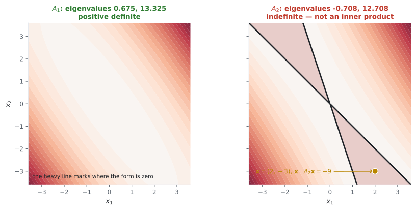
See it move

The first sketch is Example 3.4 with the broken entry on a knob. The background is the quadratic form $\mathbf{x}^\top\mathbf{A}\mathbf{x}$ — green where it is positive, red where it is negative — and the white curve is where it equals zero. Slide $a$ down through $4$ and watch the red wedge open.

sketch One entry, and the whole structure collapses p5.js Pause Restart

The field shows x-transpose A x for A = [[9, 6], [6, a]]. Green is positive, red is negative, and the white curve is the zero set. Above a = 4 the whole plane except the origin is green and A is an inner product. At exactly a = 4 the zero set becomes a line through the origin. Below it a negative wedge opens and A is no longer an inner product.

The second sketch is the payoff: the same two vectors, and an inner product you control. Drag the matrix entries and watch the inner product’s sign flip while the arrows do not move at all.

sketch The same two arrows, an inner product you control p5.js Pause Restart

Drag x and y, and drag the three entries of the symmetric matrix A. The readout gives x-transpose A y and the two induced lengths. The dashed grey curve is the set of vectors A calls unit length. Nothing about the arrows changes when you move A, and yet the number and even its sign do.

An inner product is a linear map’s worth of information, so the matrix stepper from Chapter 2 applies directly. Here it is on Example 3.3’s matrix — note the eigenvalues it reports, which are the definiteness test:

matrixExample 3.3's matrix, and why it qualifieslinear map on R^2

1-1-12

columns of A = images of e1, e2

det A 1area factor 1orientation preserved

1e1, e2 = (1, 0), (0, 1)          # the basis we start from2A @ e1  ==  A[:, 0]              # first column IS the image of e13A @ e2  ==  A[:, 1]              # second column IS the image of e24# linearity: A(x1 e1 + x2 e2) = x1 (A e1) + x2 (A e2)5det(A) = a*d - b*c               # signed area of the image of the unit square6A @ v = lam * v                  # an eigenvector keeps its direction

det A1A e1(1, -1)A e2(-1, 2)

basisThe plane before anything happens, with the standard basis e1 = (1, 0) and e2 = (0, 1) and the unit square they span.

Play‹›1/8⟲

Both eigenvalues are positive, so no direction gets flipped or flattened — which is exactly what positive definiteness means geometrically.

From scratch

Testing a candidate has three parts, and the third one has a good implementation and a bad one:

is_inner_product.py

import numpy as np
 
def is_inner_product(A, tol=1e-12):
    """Test the conditions of Definition 3.2 on a candidate matrix A."""
    A = np.asarray(A, dtype=float)
    checks = {}
 
    # 1. Bilinearity is automatic for x^T A y. Any matrix gives a bilinear form;
    #    that is what the matrix form of Equation 3.10 means. Nothing to test.
    checks["bilinear"] = True
 
    # 2. Symmetry.
    checks["symmetric"] = bool(np.allclose(A, A.T, atol=tol))
 
    # 3. Positive definiteness. Cholesky is the right test: it succeeds exactly
    #    when the matrix is positive definite, so there is no tolerance to pick.
    #    Comparing eigenvalues to zero needs one, and the choice is where the
    #    semidefinite boundary case slips through.
    if not checks["symmetric"]:
        checks["positive definite"] = False
    else:
        try:
            np.linalg.cholesky(A)
            checks["positive definite"] = True
        except np.linalg.LinAlgError:
            checks["positive definite"] = False
 
    return all(checks.values()), checks
 
candidates = {
    "identity (the dot product)": np.eye(3),
    "A1 from Example 3.4": [[9, 6], [6, 5]],
    "A2 from Example 3.4": [[9, 6], [6, 3]],
    "the a = 4 boundary": [[9, 6], [6, 4]],
    "non-symmetric": [[2, 0], [1, 2]],
    "Example 3.3": [[1, -1], [-1, 2]],
}
 
for name, A in candidates.items():
    ok, detail = is_inner_product(A)
    print(f"{'YES' if ok else 'no':4} {name:28} "
          f"symmetric={detail['symmetric']}  definite={detail['positive definite']}")

output

YES  identity (the dot product)   symmetric=True  definite=True
YES  A1 from Example 3.4          symmetric=True  definite=True
no   A2 from Example 3.4          symmetric=True  definite=False
no   the a = 4 boundary           symmetric=True  definite=False
no   non-symmetric                symmetric=False  definite=False
YES  Example 3.3                  symmetric=True  definite=True

Six candidates, three accepted. The instructive rejection is the fourth, and it is worth checking why the naive test disagrees:

why_cholesky.py

import numpy as np
 
boundary = np.array([[9.0, 6.0], [6.0, 4.0]])
print("eigenvalues:", np.round(np.linalg.eigvalsh(boundary), 12))
print("a >= 0 test would accept it:", bool(np.all(np.linalg.eigvalsh(boundary) >= 0)))
print("cholesky accepts it:", end=" ")
try:
    np.linalg.cholesky(boundary)
    print(True)
except np.linalg.LinAlgError:
    print(False)
 
w = np.array([2.0, -3.0])
print("but (2,-3) has squared length", float(w @ boundary @ w), "while being nonzero")

output

eigenvalues: [ 0. 13.]
a >= 0 test would accept it: True
cholesky accepts it: False
but (2,-3) has squared length 0.0 while being nonzero

The eigenvalues at the boundary are exactly $0$ and $13$, so np.all(eigvalsh(A) >= 0) returns True and a nonzero vector nevertheless has length zero. That is positive semidefiniteness, and Definition 3.2 asks for the strict version. Cholesky tests the strict version by construction — it is the test to reach for, and it happens to be about twice as fast as an eigendecomposition as well.

One more thing the run shows: the shear is rejected on symmetry, before definiteness is ever examined. It is worth knowing that its symmetric part $\tfrac{1}{2}(\mathbf{A}+\mathbf{A}^\top) = \begin{bmatrix}2 & 0.5 \\ 0.5 & 2\end{bmatrix}$ is positive definite, so the shear gives a perfectly positive quadratic form $\mathbf{x}^\top\mathbf{A}\mathbf{x}$ while still failing to be an inner product. Definiteness of the form is not enough; the matrix itself has to be symmetric, or the two arguments are not interchangeable.

On real data

figure Example 3.4, as a surface matplotlib

A1 has eigenvalues 0.675 and 13.325 and never goes negative. A2 has eigenvalues -0.708 and 12.708, and the shaded wedge is where a vector would have negative squared length. The marked point is the book's witness, at which the form equals exactly -9.

figure Three inner products, three meanings of length one matplotlib

The point (1, 1) has length 1.4142 under the dot product, exactly 1.0000 under the book's Equation 3.19, and 1.7321 under diag(2, 1). It lies exactly on the amber curve, which is what makes it a unit vector under that inner product and not under the others.

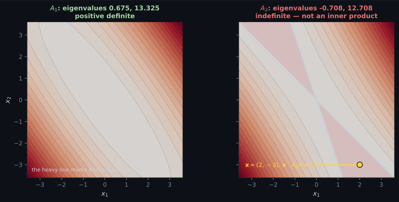
Reading the plot

From the surface plot. The interesting feature of $\mathbf{A}_2$‘s panel is not that a negative region exists but that it is a wedge through the origin, not a bounded blob. Positive definiteness is a statement about directions rather than about magnitudes: the form is homogeneous of degree two, so if it is negative at $\mathbf{x}$ it is negative along the whole line through $\mathbf{x}$, scaled by $\lambda^2$. The negative eigenvalue $-0.708204$ is the value of the form at its own eigenvector, and that is the most negative value any unit vector can produce. The book’s witness $(2,-3)$ is a different direction in the same wedge — normalised, it scores $-0.692308$, which is close to the extreme without being it.

Note also that $\mathbf{A}_2$‘s largest eigenvalue is $12.708$ — comfortably positive. A single negative eigenvalue among positives is enough. There is no “mostly positive definite”.

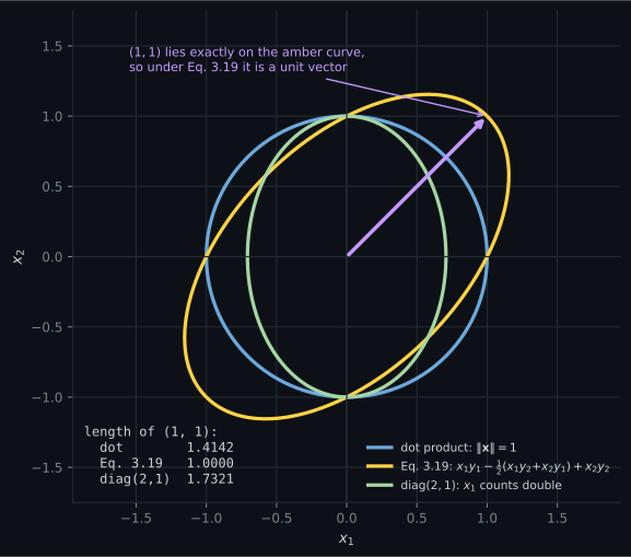
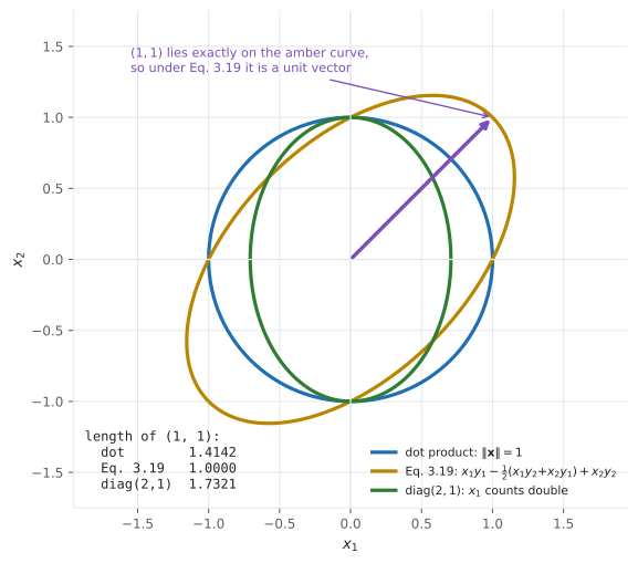
From the unit sets. The three curves have the same centre and enclose the point $(1,1)$ to different depths, which is the visual form of the statement that the same vector has three lengths. More usefully: the shape tells you what the inner product cares about. The axis-aligned ellipse of $\mathrm{diag}(2,1)$ is narrow in $x_1$, meaning $x_1$ is expensive — a small step in $x_1$ counts as much length as a bigger step in $x_2$. The tilted ellipse of Equation 3.19 is stretched along the diagonal $x_1 = x_2$, meaning that agreement between the coordinates is cheap: moving both together costs less length than moving one alone. That is what a negative off-diagonal entry does, and it is exactly the structure a covariance matrix has when two features are positively correlated.

Pitfalls

Positive diagonal is not positive definite

$\mathbf{A}_2 = \begin{bmatrix}9&6\\6&3\end{bmatrix}$ has both diagonal entries positive and is still not an inner product. Checking the diagonal is a necessary condition and people routinely treat it as sufficient. The determinant of every leading submatrix being positive (Sylvester’s criterion) is the sufficient version; Cholesky is the sufficient version you should actually run.

Semidefinite is not definite, and the difference is not academic

At $a = 4$ the matrix has eigenvalues $0$ and $13$. Every eigenvalue is non-negative, so np.all(eigvalsh(A) >= 0) returns True. But the vector $(2,-3)$ then has squared length exactly zero without being the zero vector, so the induced “norm” is not positive definite and the geometry falls apart. Test with Cholesky, or test > 0 rather than >= 0 — and if you do the latter, be honest about the tolerance you are choosing.

Symmetry is a real requirement, not a convenience

For a non-symmetric $\mathbf{A}$, the form $\mathbf{x}^\top\mathbf{A}\mathbf{y}$ is still bilinear, and $\mathbf{x}^\top\mathbf{A}\mathbf{x}$ is still well defined — but $\langle\mathbf{x},\mathbf{y}\rangle \neq \langle\mathbf{y},\mathbf{x}\rangle$, so “the angle between $\mathbf{x}$ and $\mathbf{y}$” would depend on the order you named them. Note also that only the symmetric part of $\mathbf{A}$ affects $\mathbf{x}^\top\mathbf{A}\mathbf{x}$, so a non-symmetric matrix and its symmetrisation $\tfrac{1}{2}(\mathbf{A}+\mathbf{A}^\top)$ give the same quadratic form — which is why the definiteness test starts by insisting on symmetry.

An inner product is bilinear, which means it is not linear

$\langle 2\mathbf{x}, 2\mathbf{y}\rangle = 4\langle\mathbf{x},\mathbf{y}\rangle$. Doubling both arguments quadruples the result. This trips people up when normalising: scaling a dataset by $c$ scales its Gram matrix by $c^2$, not by $c$.

Estimated covariance matrices are often only semidefinite

The natural inner product on centred data is $\langle\mathbf{x},\mathbf{y}\rangle = \mathbf{x}^\top \Sigma^{-1}\mathbf{y}$, and $\Sigma$ estimated from $n$ samples in $d$ dimensions has rank at most $\min(n-1, d)$. With fewer samples than features it is singular, $\Sigma^{-1}$ does not exist, and no amount of care about the mathematics will save the call. This is why practical code adds a ridge $\Sigma + \varepsilon\mathbf{I}$ — the same “jitter term” the book mentions in §3.8.2.

Compare

candidate	matrix	inner product?	why
dot product	$\mathbf{I}$	yes	symmetric, all eigenvalues $1$
weighted dot	$\mathrm{diag}(w_1,\dots,w_n)$, $w_i > 0$	yes	symmetric, eigenvalues are the weights
Example 3.3	$\begin{bmatrix}1&-1\\-1&2\end{bmatrix}$	yes	eigenvalues $0.382$, $2.618$
Mahalanobis	$\Sigma^{-1}$ for invertible $\Sigma$	yes	a covariance matrix of full rank is SPD, and so is its inverse
$\mathbf{A}_1$	$\begin{bmatrix}9&6\\6&5\end{bmatrix}$	yes	completing the square gives a sum of two squares
the $a=4$ boundary	$\begin{bmatrix}9&6\\6&4\end{bmatrix}$	no	semidefinite: $(2,-3)$ has squared length $0$
$\mathbf{A}_2$	$\begin{bmatrix}9&6\\6&3\end{bmatrix}$	no	$(2,-3)$ has squared length $-9$
a shear	$\begin{bmatrix}2&0\\1&2\end{bmatrix}$	no	not symmetric

pch.quizTag Check your understanding

1. Theorem 3.5 says something stronger than 'matrices give inner products'. What is the extra content?

   A That inner products are always computable B That the correspondence runs both ways: every inner product on a finite-dimensional real vector space with a fixed basis IS x-transpose A y for some symmetric positive definite A, so there are no other kinds C That A must be the identity D That every symmetric matrix gives an inner product
   pch.quizShowAnswer

   B — That the correspondence runs both ways: every inner product on a finite-dimensional real vector space with a fixed basis IS x-transpose A y for some symmetric positive definite A, so there are no other kinds — The 'if and only if' is what makes the test practical: checking a candidate reduces to checking whether one matrix is SPD, with no exotic cases to worry about. Note that plain symmetry is not enough — A2 of Example 3.4 is symmetric and fails.

2. A2 = [[9, 6], [6, 3]] has positive diagonal entries and a trivial-looking structure. Why is it not an inner product?

   A Because it is not symmetric B Because completing the square gives (3x1 + 2x2)^2 minus x2^2, and the witness (2, -3) makes that minus 9 — a nonzero vector with negative squared length C Because its entries are too large D Because its determinant is not 1
   pch.quizShowAnswer

   B — Because completing the square gives (3x1 + 2x2)^2 minus x2^2, and the witness (2, -3) makes that minus 9 — a nonzero vector with negative squared length — The determinant is -9 and the eigenvalues are -0.708 and 12.708. One negative eigenvalue among positive ones is enough; there is no partial credit for definiteness.

3. Why does the from-scratch code use Cholesky rather than comparing eigenvalues to zero?

   A Cholesky is more accurate for eigenvalues B Because Cholesky tests definiteness exactly, whereas an eigenvalue comparison needs a tolerance — and at the a = 4 boundary the eigenvalues are 0 and 13, so a >= 0 test wrongly accepts a matrix that Definition 3.2 rejects C Because eigenvalues are not defined for non-symmetric matrices D Cholesky also checks symmetry
   pch.quizShowAnswer

   B — Because Cholesky tests definiteness exactly, whereas an eigenvalue comparison needs a tolerance — and at the a = 4 boundary the eigenvalues are 0 and 13, so a >= 0 test wrongly accepts a matrix that Definition 3.2 rejects — It is also about twice as fast, but the correctness argument is the one that matters. Semidefinite is not definite, and the a = 4 case is exactly where the two tests disagree.

4. Under the dot product, x = (1, 2) and y = (3, -1) have inner product +1. Under Example 3.3's inner product the value is -6. What should you conclude?

   A One of the two calculations is wrong B Nothing follows — the two numbers measure different things, and whether two vectors 'agree' is a statement relative to a chosen inner product, including its sign C The vectors must be orthogonal D Example 3.3 is not a valid inner product
   pch.quizShowAnswer

   B — Nothing follows — the two numbers measure different things, and whether two vectors 'agree' is a statement relative to a chosen inner product, including its sign — Example 3.3's matrix has eigenvalues 0.382 and 2.618, so it is a perfectly valid inner product. The sign flip is the point: cosine similarity, orthogonality and angle all inherit this relativity, which is what the next two pages develop.

🧪 Try It Yourself

Exercise 1 – Test the three conditions

pch.exerciseTag pch.exerciseTitle

Exercise 2 – The worst direction, and the book’s witness

pch.exerciseTag pch.exerciseTitle

Exercise 3 – Bilinearity, symmetry, definiteness, all measured

pch.exerciseTag pch.exerciseTitle

Exercise 4 – The Gram matrix of a basis

pch.exerciseTag pch.exerciseTitle

Exercise 5 – Where does it break?

pch.exerciseTag pch.exerciseTitle

Recall card

• An inner product is a bilinear, symmetric, positive definite function of two vectors, and those three words are the entire definition.
• Bilinear means linear in each argument separately — scaling both arguments scales the result by the square, so an inner product is not a linear map.
• Theorem 3.5 is an if and only if: every inner product on a finite-dimensional real space is x-transpose A y for a symmetric positive definite A, and every such A gives one.
• Positive definiteness is what makes the induced norm real, since length is the square root of the inner product of a vector with itself.
• A positive diagonal is necessary but not sufficient — the book’s second matrix of Example 3.4 has both diagonal entries positive and a witness of squared length minus nine.
• Semidefinite is not definite: at the boundary value the eigenvalues are zero and thirteen, and a nonzero vector has length zero. Test with Cholesky, not with eigenvalues compared to zero.
• The dot product is the case where the matrix is the identity, which is why it treats coordinates as independent and equally weighted.

Next: Lengths and Distances — the first two things the inner product hands you for free.