The Dual Support Vector Machine

Everything so far has been written in terms of $\mathbf{w}$, which lives in $\mathbb{R}^D$. That is the primal SVM, and its size grows with the number of features. Section 12.3 rewrites the same problem in terms of one multiplier per example — and in doing so produces the form that Section 12.4 can kernelise.

The Lagrangian and its three derivatives

Attach $\alpha_n \geq 0$ to the margin constraint 12.26b and $\gamma_n \geq 0$ to the non-negativity constraint 12.26c:

$$\mathfrak{L}(\mathbf{w}, b, \boldsymbol\xi, \boldsymbol\alpha, \boldsymbol\gamma) = \tfrac12\lVert\mathbf{w}\rVert^2 + C\sum_{n=1}^{N}\xi_n - \sum_{n=1}^{N}\alpha_n\big(y_n(\langle\mathbf{w},\mathbf{x}_n\rangle + b) - 1 + \xi_n\big) - \sum_{n=1}^{N}\gamma_n\xi_n \qquad \text{(12.34)}$$

Differentiating in the three primal variables:

$$\frac{\partial\mathfrak{L}}{\partial\mathbf{w}} = \mathbf{w}^\top - \sum_n \alpha_n y_n \mathbf{x}_n^\top, \qquad \frac{\partial\mathfrak{L}}{\partial b} = -\sum_n \alpha_n y_n, \qquad \frac{\partial\mathfrak{L}}{\partial\xi_n} = C - \alpha_n - \gamma_n \qquad \text{(12.35)–(12.37)}$$

Setting the first to zero gives the result the rest of the chapter rests on:

$$\mathbf{w} = \sum_{n=1}^{N}\alpha_n y_n \mathbf{x}_n \qquad \text{(12.38)}$$

the representer theorem — the optimal weight vector is a linear combination of the training examples. Setting the second to zero adds $\sum_n \alpha_n y_n = 0$, which makes it an affine combination. Setting the third to zero and using $\gamma_n \geq 0$ gives $\alpha_n \leq C$.

Substituting back eliminates $\mathbf{w}$, $b$ and $\boldsymbol\xi$ entirely (Equations 12.39, 12.40) and leaves

$$\min_{\boldsymbol\alpha}\ \tfrac12\sum_{i=1}^{N}\sum_{j=1}^{N} y_i y_j \alpha_i \alpha_j \langle\mathbf{x}_i, \mathbf{x}_j\rangle - \sum_{i=1}^{N}\alpha_i \quad\text{subject to}\quad \sum_i y_i\alpha_i = 0, \quad 0 \leq \alpha_i \leq C \qquad \text{(12.41)}$$

The examples appear only through $\langle\mathbf{x}_i, \mathbf{x}_j\rangle$. That is the whole point of the exercise, and page 1208 collects the winnings.

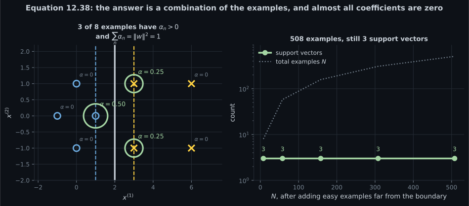
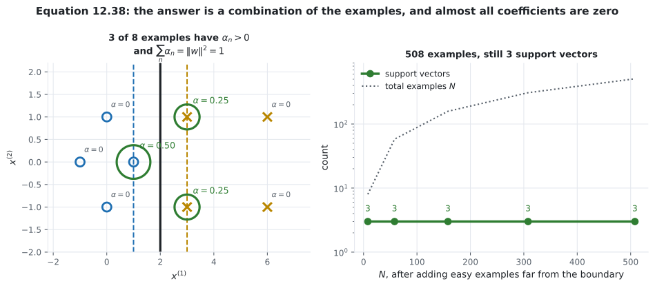
The running example, exactly

The eight-point dataset has a dual solution that can be written down by hand. With $\mathbf{w} = (1, 0)$ and support vectors $(3, 1)$, $(3, -1)$ and $(1, 0)$, Equation 12.38 and the constraint $\sum_n \alpha_n y_n = 0$ give $\alpha_0 = \alpha_1 = \tfrac14$ and $\alpha_4 = \tfrac12$.

the_dual.py

import numpy as np
from scipy.optimize import minimize
 
X = np.array([[3.0,  1.0], [3.0, -1.0], [6.0,  1.0], [6.0, -1.0],
              [1.0,  0.0], [0.0,  1.0], [0.0, -1.0], [-1.0, 0.0]])
Y = np.array([ 1.0,  1.0,  1.0,  1.0,  -1.0, -1.0, -1.0, -1.0])
BIG = 1e6                                # stands in for the hard margin
 
def dual(XX, YY, C, tries=25):
    H = (YY[:, None] * YY[None, :]) * (XX @ XX.T)       # Y K Y
    out, bv = None, np.inf
    for s in range(tries):
        rg = np.random.default_rng(s)
        a0 = np.clip(np.abs(rg.normal(0.3, 0.3, len(XX))), 0, C)
        r = minimize(lambda a: 0.5 * a @ H @ a - a.sum(), a0,
                     jac=lambda a: H @ a - 1.0,
                     bounds=[(0.0, C)] * len(XX),
                     constraints=[{"type": "eq", "fun": lambda a: YY @ a,
                                   "jac": lambda a: YY}],
                     method="SLSQP", options={"maxiter": 30000, "ftol": 1e-14})
        if r.success and r.fun < bv - 1e-13:
            bv, out = r.fun, np.clip(r.x, 0.0, C)
    return out
 
a = dual(X, Y, BIG)
w = a * Y @ X                                            # Equation 12.38
print(f"alpha            : {np.round(a, 8)}")
print(f"w = sum a y x    : {np.round(w, 8)}")
print(f"sum y_n alpha_n  : {Y @ a:.3e}")
print(f"support vectors  : {list(np.where(a > 1e-9)[0])}")

text

alpha            : [0.25 0.25 0.   0.   0.5  0.   0.   0.  ]
w = sum a y x    : [1. 0.]
sum y_n alpha_n  : -5.306e-16
support vectors  : [0, 1, 4]

The largest deviation from the exact $(\tfrac14, \tfrac14, 0, 0, \tfrac12, 0, 0, 0)$ is $1.075\times10^{-8}$, and $\mathbf{w}$ recovers the primal answer to $1.950\times10^{-8}$.

An identity the book does not state

At a hard-margin optimum,

$$\lVert\mathbf{w}\rVert^2 = \sum_{n=1}^{N}\alpha_n = \frac{1}{r^2}$$

so the total dual mass is the inverse squared margin. Here all three are $1.000000$. Checked across $200$ random separable datasets in $2$ to $4$ dimensions: worst deviation $4.782\times10^{-8}$, and the dual’s $\mathbf{w}$ matches the primal’s to $1.208\times10^{-7}$.

It follows in one line from Equations 12.38 and 12.15: at the optimum every support vector has $y_n f(\mathbf{x}_n) = 1$, so $\lVert\mathbf{w}\rVert^2 = \langle\mathbf{w}, \sum_n \alpha_n y_n \mathbf{x}_n\rangle = \sum_n \alpha_n y_n \langle\mathbf{w},\mathbf{x}_n\rangle = \sum_n \alpha_n(1 - y_n b) = \sum_n\alpha_n$, the last step using $\sum_n \alpha_n y_n = 0$.

A wide margin means small multipliers — which is the dual’s way of saying the same thing the primal says by minimising $\lVert\mathbf{w}\rVert^2$.

Sparsity is the point

The book’s remark is short: “The examples $\mathbf{x}_n$, for which the corresponding parameters $\alpha_n = 0$, do not contribute to the solution $\mathbf{w}$ at all. The other examples, where $\alpha_n > 0$, are called support vectors.”

Measured from both directions:

sparsity.py

sv = a > 1e-9
a2 = dual(X[sv], Y[sv], BIG)              # keep ONLY the support vectors
print(f"refit on {int(sv.sum())} points : alpha = {np.round(a2, 8)}")
print(f"  w = {np.round(a2 * Y[sv] @ X[sv], 8)}, gap "
      f"{np.linalg.norm(a2 * Y[sv] @ X[sv] - w):.3e}")
 
rg = np.random.default_rng(7)             # now ADD 500 easy examples
XL = np.vstack([X, rg.uniform([20, -5], [40, 5], (250, 2)),
                rg.uniform([-40, -5], [-20, 5], (250, 2))])
YL = np.r_[Y, np.ones(250), -np.ones(250)]
aL = dual(XL, YL, BIG, tries=6)
print(f"N = {len(XL)} : support vectors {int((aL > 1e-9).sum())}, "
      f"w gap {np.linalg.norm(aL * YL @ XL - w):.3e}")
print(f"  alpha mass on the 500 extras : {aL[8:].sum():.3e}")

text

refit on 3 points : alpha = [0.25 0.25 0.5 ]
  w = [ 1. -0.], gap 1.950e-08
N = 508 : support vectors 3, w gap 6.238e-09
  alpha mass on the 500 extras : 8.289e-12

Five of eight examples can be deleted without changing the answer, and five hundred more can be added without changing it either. The five hundred extras collectively carry $8.289\times10^{-12}$ of dual mass. This is the same property page 1205 measured from the primal side: a point beyond its margin has zero hinge loss, and here it has zero multiplier.

figure Equation 12.38: the answer is a combination of the examples, and almost all coefficients are zero matplotlib

The ringed areas are the multipliers, and they sum to ||w||² = 1. The right panel is the practical consequence: prediction cost scales with the number of support vectors, not with N.

Recovering b, and a wrinkle in the remark

The dual returns $\boldsymbol\alpha$, and Equation 12.38 returns $\mathbf{w}$ — but $b$ was eliminated. For an example on the margin, $\langle\mathbf{w}^*, \mathbf{x}_n\rangle + b = y_n$, so

$$b^* = y_n - \langle\mathbf{w}^*, \mathbf{x}_n\rangle \qquad \text{(12.42)}$$

text

from example 0 : b = -1.999999981275
from example 1 : b = -1.999999949778
from example 4 : b = -1.999999988509
the primal's b*: -2.0

The book adds: “In principle, there may be no examples that lie exactly on the margin. In this case, we should compute $\lvert y_n - \langle\mathbf{w}^*,\mathbf{x}_n\rangle\rvert$ for all support vectors and take the median value to be the value of $b^*$.”

That rule as written discards the sign. Taking the median of an absolute value returns a non-negative number, and $b^*$ here is $-2$:

$C$	$b$ from Equation 12.42	the median-of-absolute rule
$0.2$	$-1.000000$	$+1.000000$
$0.5$	$-2.000000$	$+2.000000$
$1.0$	$-2.000000$	$+2.000000$
$5.0$	$-2.000000$	$+2.000000$

The magnitudes agree to $8.1\times10^{-9}$ or better, so the intent is clear and the fix is to drop the absolute value — take the median of $y_n - \langle\mathbf{w}^*,\mathbf{x}_n\rangle$ itself.

The margin note is a one-way implication

The book’s side note reads:

It turns out that examples that lie exactly on the margin are examples whose dual parameters lie strictly inside the box constraints, $0 < \alpha_i < C$.

The KKT conditions give three implications:

condition	consequence
$\alpha_n = 0$	$y_n f(\mathbf{x}_n) \geq 1$ — at or beyond the margin
$0 < \alpha_n < C$	$y_n f(\mathbf{x}_n) = 1$ — exactly on the margin
$\alpha_n = C$	$y_n f(\mathbf{x}_n) \leq 1$ — at or inside the margin

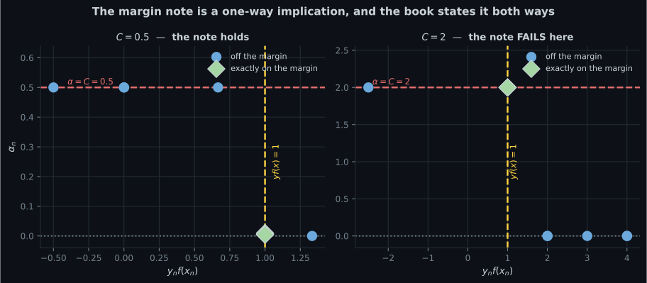
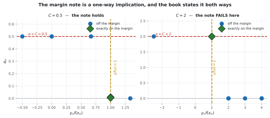
The middle row is the note’s claim read left to right, and it is correct. The note is phrased the other way round — examples on the margin are examples with $0 < \alpha_i < C$ — and that direction is false, because the third row also permits $y_n f(\mathbf{x}_n) = 1$ exactly.

text

  C = 0.5   (b from the primal: -1.000000)
    n       x_n    y     alpha    y f(x)              position
    0   [3.  1.]   +1  0.500000 -0.000000   inside / wrong side
    2   [6.  1.]   +1  0.009204  1.000000         ON the margin
    3   [6. -1.]   +1  0.004685  1.000000         ON the margin
    7   [-1. 0.]   -1  0.000000  1.333333     beyond the margin
      on the margin : alpha in [0.004685, 0.009204]   -- strictly inside
 
  C = 2.0   (b from the primal: -2.000000)
    n       x_n    y     alpha    y f(x)              position
    0   [3.  1.]   +1  2.000000  1.000000         ON the margin
    1   [3. -1.]   +1  2.000000  1.000000         ON the margin
    4   [1.  0.]   -1  2.000000  1.000000         ON the margin
    8   [4.5 0.]   -1  2.000000 -2.500000   inside / wrong side
      on the margin : alpha in [2.000000, 2.000000]   -- AT the bound

At $C = 2$, three examples sit exactly on the margin with $\alpha_n = C$ — at the box bound, not strictly inside it. This is not a solver artefact: the optimum is unique there. Writing $\alpha_0 = \alpha_1 = t$, $\alpha_4 = s$, $\alpha_8 = u$, the constraints force $s = 2t - u$ and $4t - 3.5u = 1$, and the dual objective is $\tfrac12\lVert\mathbf{w}\rVert^2 - \sum\alpha_n$ with $\sum\alpha_n = 1 + 3.5u$. Maximising that pushes $u$ to its bound $C = 2$, giving $(t, s, u) = (2, 2, 2)$ — all three at the bound, and $\sum\alpha_n = 8$, matching the measured dual value of $-7.5 = 0.5 - 8$.

figure The margin note is a one-way implication, and the book states it both ways matplotlib

Left, the textbook picture the note describes. Right, the same data at C = 2, where the on-margin examples have their multipliers pinned at the box bound. The correct statement runs only one way: strictly inside the box implies on the margin, not the converse.

Strong duality, measured

Equation 12.41 is the negated Lagrangian dual, so the primal optimum equals minus the dual optimum. Across five values of $C$ on the non-separable data:

$C$	primal objective	$-$ dual objective	gap
$0.2$	$0.82222222$	$0.82222222$	$9.992\times10^{-16}$
$1.0$	$3.87500000$	$3.87500000$	$1.332\times10^{-15}$
$5.0$	$18.00000000$	$18.00000000$	$1.847\times10^{-13}$

Zero duality gap, to machine precision. It holds because the primal is convex with affine constraints — Slater’s condition — and it is what makes solving the dual instead of the primal legitimate rather than merely convenient.

pch.quizTag Check your understanding

1. A That the coefficients are positive B That the coefficients sum to one C That sum of y_n alpha_n is zero, which makes it an affine combination rather than merely a linear one D That w has unit norm
   pch.quizShowAnswer

   C — That sum of y_n alpha_n is zero, which makes it an affine combination rather than merely a linear one

2. A Because the extras were duplicates B Because a point beyond its margin has zero hinge loss in the primal and zero multiplier in the dual — it contributes nothing to Equation 12.38 C Because the solver ignored them D Because C was too large
   pch.quizShowAnswer

   B — Because a point beyond its margin has zero hinge loss in the primal and zero multiplier in the dual — it contributes nothing to Equation 12.38

3. A The median should be a mean B It should use all examples, not just support vectors C The absolute value discards the sign, so the rule returns a non-negative number — on this data b* is -2 and the rule returns +2 D Nothing; it is exact
   pch.quizShowAnswer

   C — The absolute value discards the sign, so the rule returns a non-negative number — on this data b* is -2 and the rule returns +2

4. A The measurement must be wrong; KKT forbids it B The note's implication holds in one direction only: 0 < alpha < C implies on the margin, but an on-margin example may also have alpha = C. The note is phrased as the converse C It shows C was chosen badly D It shows the problem is not convex
   pch.quizShowAnswer

   B — The note's implication holds in one direction only: 0 < alpha < C implies on the margin, but an on-margin example may also have alpha = C. The note is phrased as the converse

Exercises

Exercise 1 – Solve the dual and recover w

pch.exerciseTag pch.exerciseTitle

Exercise 2 – Delete everything that is not a support vector

pch.exerciseTag pch.exerciseTitle

Exercise 3 – Test the margin note in both directions

pch.exerciseTag pch.exerciseTitle

Recall card

• The primal SVM’s size grows with the number of features; the dual’s grows with the number of examples. Section 12.3 rewrites the same problem in terms of one multiplier per example.
• Equation 12.38 is the representer theorem: the optimal weight vector is a linear combination of the training examples, and the constraint from the derivative in b makes it an affine one.
• In the dual the examples appear only through their inner products. That is what makes Section 12.4’s kernel substitution a one-line change.
• On the running example the dual is exact: the multipliers are a quarter, a quarter and a half, and they recover w = (1, 0) to 2e-08.
• An identity the book does not state: the total dual mass equals the squared norm of w, which is the inverse squared margin. Verified to 4.8e-08 across 200 random datasets. A wide margin means small multipliers.
• Sparsity is the point. Five of the eight examples can be deleted without changing the answer, and 500 easy ones can be added without changing it either — they carry 8.3e-12 of dual mass between them.
• That is the dual’s version of page 1205’s finding: a point beyond its margin has zero hinge loss and zero multiplier.
• Recovering b needs an example on the margin, and the book’s fallback rule takes a median of absolute values — which discards the sign and returns plus two where the answer is minus two.
• Strong duality holds to machine precision, because the primal is convex with affine constraints. That is what makes solving the dual instead of the primal legitimate rather than merely convenient.
• The book’s margin note about the box constraints runs only one way. Strictly inside the box implies exactly on the margin; the converse is false, and at C = 2 three on-margin examples sit at the bound.
• That case is a unique optimum, not solver noise — the constraints force a single feasible family and the objective pushes the multipliers to the bound.

Next: The Convex Hull View — §12.3.2, the same dual reached by a completely different geometric argument.