Updating the Covariances

The second update runs the same argument as the first, with a harder derivative. §11.2.3 spends three pages on matrix calculus to reach a formula you could have guessed — and the interesting part is what it does to page 1101’s decomposition once it is in place.

What you’ll learn

• Theorem 11.2, Equation 11.30, and Example 11.4 reproduced: $1 \to 0.144000$, $0.2 \to 0.438492$, $3 \to 1.526594$, rounding to the book’s $0.14$, $0.44$, $1.53$.
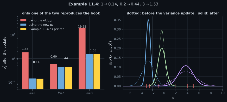
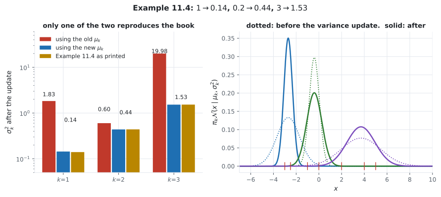
• Which $\boldsymbol\mu_k$ Equation 11.30 means. Written with the old means it gives $1.83$, $0.60$, $19.98$; with the just-updated means it gives the book’s numbers. The equation does not say, and the answer differs by a factor of $13$ on the third component.
• Equations 11.31–11.38: the proof, and the single cancellation that turns a messy stationarity condition into a weighted second moment. Measured to $2.2\times10^{-16}$.
• Why no positive-definiteness repair is ever needed: measured over $60{,}000$ variances from random responsibilities, zero negative results.
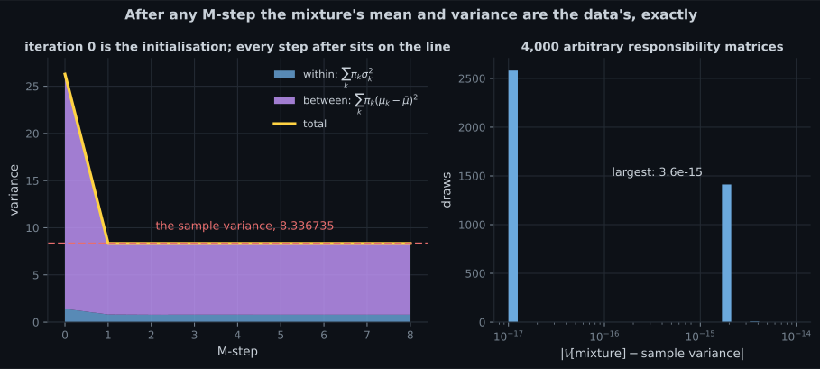
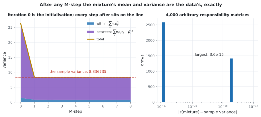
• An invariant the book does not state, stronger than page 1104’s: after any M-step, the mixture’s variance equals the sample variance exactly — measured to $3.6\times10^{-15}$ over $20{,}000$ arbitrary responsibility matrices, and for every $K$ from $2$ to $10$.
• So EM moves variance from between components to within them and back, with the total pinned — page 1101’s decomposition, in motion.
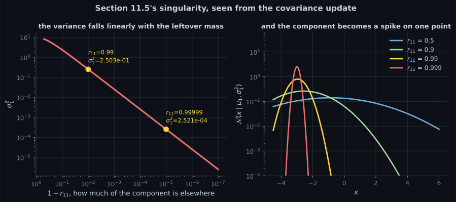
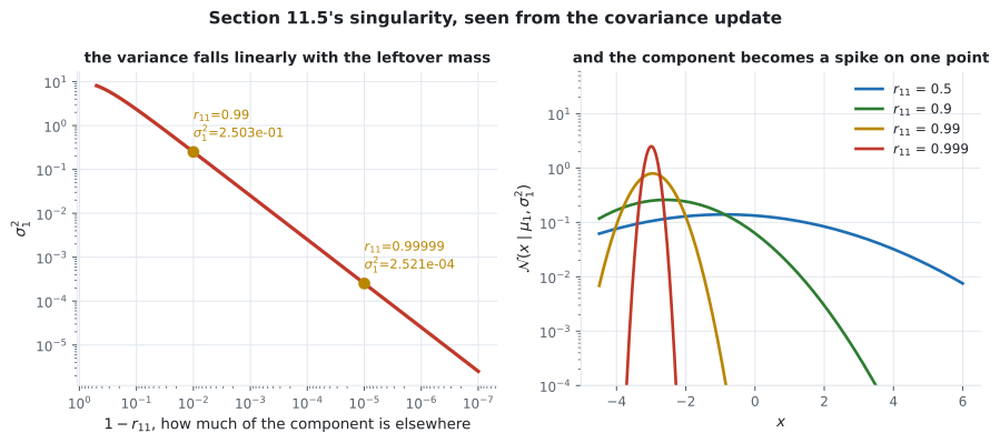
• And the singularity from the covariance side: as a component’s responsibility concentrates on one point, $\sigma_k^2 \to 0$ linearly in the leftover mass.

Intuition: the same weighted average, one moment up

Page 1104’s update was $\sum_n w_n x_n$ with $w_n = r_{nk}/N_k$. This one is $\sum_n w_n(x_n-\mu_k)^2$ — the same weights, applied to squared deviations instead of positions.

That is the whole of Theorem 11.2. The three pages of matrix calculus exist to show that the derivative of $\log\det$ and the derivative of a quadratic form conspire to leave exactly this, with the inverse covariances cancelling as they did for the means.

diagram The same skeleton, one moment higher mermaid

  flowchart TD
  A["d p / d Sigma_k, Equations 11.32 to 11.35"]
  A -->|"chain rule through 1/p(x_n)"| B["r_nk appears again
Equation 11.36b"]
  B --> C["N_k Sigma^-1 = Sigma^-1 (sum r (x-mu)(x-mu)') Sigma^-1
Equation 11.37a"]
  C -->|"cancel Sigma^-1 once from each side"| D["N_k I = (sum r (x-mu)(x-mu)') Sigma^-1
Equation 11.37b"]
  D --> E["Sigma_k = (1/N_k) sum_n r_nk (x_n-mu_k)(x_n-mu_k)'
Equation 11.30"]
  E --> F["a weighted second moment:
always positive semi-definite"]

§11.2.3 Theorem 11.2

Theorem 11.2 (Updates of the GMM Covariances). The update of the covariance parameters $\boldsymbol\Sigma_k$ of the GMM is given by

$$\boldsymbol\Sigma_k^{\text{new}} = \frac{1}{N_k}\sum_{n=1}^{N} r_{nk}(\mathbf{x}_n-\boldsymbol\mu_k)(\mathbf{x}_n-\boldsymbol\mu_k)^\top \qquad \text{(11.30)}$$

The proof needs two identities from Chapter 5 — Equation 5.101 for $\partial\det(\boldsymbol\Sigma)^{-1/2}$ and Equation 5.106 for the derivative of the quadratic form — which combine into

$$\frac{\partial p(\mathbf{x}_n\mid\boldsymbol\theta)}{\partial\boldsymbol\Sigma_k} = \pi_k\mathcal{N}(\mathbf{x}_n\mid\boldsymbol\mu_k,\boldsymbol\Sigma_k)\cdot\left(-\tfrac12\big(\boldsymbol\Sigma_k^{-1}-\boldsymbol\Sigma_k^{-1}(\mathbf{x}_n-\boldsymbol\mu_k)(\mathbf{x}_n-\boldsymbol\mu_k)^\top\boldsymbol\Sigma_k^{-1}\big)\right) \qquad \text{(11.35)}$$

and, after the responsibilities reappear and the derivative is set to zero,

$$N_k\boldsymbol\Sigma_k^{-1} = \boldsymbol\Sigma_k^{-1}\left(\sum_n r_{nk}(\mathbf{x}_n-\boldsymbol\mu_k)(\mathbf{x}_n-\boldsymbol\mu_k)^\top\right)\boldsymbol\Sigma_k^{-1} \qquad \text{(11.37a)}$$

Cancelling $\boldsymbol\Sigma_k^{-1}$ once from each side gives Equation 11.37b and then Equation 11.30. In one dimension, checked on the book’s numbers:

	$k=1$	$k=2$	$k=3$
$N_k/\sigma_k^2$	$14.286319$	$4.581629$	$1.921770$
$\left(\sum_n r_{nk}(x_n-\mu_k)^2\right)/(\sigma_k^2)^2$	$14.286319$	$4.581629$	$1.921770$

with a gap of $2.2\times10^{-16}$.

Which mean does Equation 11.30 use?

The equation writes $\boldsymbol\mu_k$ with no superscript. It matters:

	$k=1$	$k=2$	$k=3$
with the old means $(-4, 0, 8)$	$1.830803$	$0.601232$	$\mathbf{19.979741}$
with the new means from Equation 11.20	$\mathbf{0.144000}$	$\mathbf{0.438492}$	$\mathbf{1.526594}$
Example 11.4 as printed	$0.14$	$0.44$	$1.53$

figure The equation does not say which mean, and the two answers differ by a factor of 13 matplotlib

Example 11.4 follows Example 11.3, and the book's Figure 11.6(a) is its Figure 11.5(b) — so the means have already moved. Using them reproduces the printed variances; using the pre-update means gives 19.98 for the third component instead of 1.53.

This is the ordering that makes EM what it is

Both readings are defensible from Equation 11.30 alone, and the difference is not small. The book resolves it by ordering the examples — §11.2.2 then §11.2.3, with Figure 11.6(a) repeating Figure 11.5(b) — and §11.3’s algorithm makes it explicit: the M-step reestimates $\boldsymbol\mu_k, \boldsymbol\Sigma_k, \pi_k$ in that order, each using the values already computed in the same step.

Using the stale means is not merely different, it is worse: it measures spread about a point the component has already left. The third component’s $19.98$ is the squared distance from $8$ to data that lives below $5$.

Always positive semi-definite, for free

Equation 11.30 is $\sum_n w_n \mathbf{v}_n\mathbf{v}_n^\top$ with $w_n \geq 0$ — a non-negative combination of rank-one positive semi-definite matrices. So the result is positive semi-definite by construction, with no projection, clipping or eigenvalue repair.

Measured in one dimension over $20{,}000$ random responsibility matrices ($60{,}000$ variances):

	value
variances that came out negative	$\mathbf{0}$
smallest value seen	$1.508415$

Compare page 1005’s measurement, where eigh on a badly conditioned $\mathbf{X}\mathbf{X}^\top$ returned $18$ negative eigenvalues of $200$. Here the structure of the update guarantees what the numerics there could not.

The invariant, one moment up

Page 1104 measured $\sum_k N_k\mu_k = \sum_n x_n$. The same swap-the-summation argument, applied to second moments, gives more:

$$\sum_k \pi_k\left(\sigma_k^2 + \mu_k^2\right) = \frac{1}{N}\sum_n x_n^2$$

so the fitted mixture’s variance is the sample variance, exactly, after any M-step:

	value
sample mean	$0.642857142857$
sample variance	$8.336734693878$
worst $\lvert$mixture mean $-$ sample mean$\rvert$, $20{,}000$ random $\mathbf{R}$	$5.6\times10^{-16}$
worst $\lvert$mixture variance $-$ sample variance$\rvert$	$\mathbf{3.6\times10^{-15}}$

and it does not depend on $K$:

$K$	worst mean gap	worst variance gap
$2$	$5.6\times10^{-16}$	$3.6\times10^{-15}$
$3$	$5.6\times10^{-16}$	$3.6\times10^{-15}$
$5$	$6.7\times10^{-16}$	$3.6\times10^{-15}$
$10$	$5.6\times10^{-16}$	$1.8\times10^{-15}$

figure The total never moves again after the first M-step matplotlib

Iteration 0 is the book's initialisation, whose mixture variance is 26.288889 — it has not been fitted to anything yet. Every M-step after that lands the total exactly on the sample variance, 8.336735, and all subsequent movement is variance migrating between the two bands.

What EM is actually doing, in one sentence

Page 1101 split a mixture’s variance into a within-component part and a between-component part. This invariant says their sum is fixed the moment you fit. So:

M-step	within	between	total
$0$ (the initialisation)	$1.400000$	$24.888889$	$26.288889$
$1$	$0.807977$	$7.528757$	$\mathbf{8.336735}$
$2$	$0.783119$	$7.553616$	$\mathbf{8.336735}$
$6$	$0.791038$	$7.545697$	$\mathbf{8.336735}$

EM cannot make the model narrower or wider than the data — it can only decide how much of the spread is “different components” and how much is “width within a component.” That is the trade it is running, and the log-likelihood is what scores it.

It also explains the failure mode of page 1102 from a new angle: a component collapsing to zero width pushes all its variance into the between term, which is free, while the within term goes to zero. The invariant is satisfied and the model is useless.

The singularity, from this side

As a component’s responsibility concentrates on a single point, Equation 11.30’s weighted second moment about that point collapses:

$r_{11}$	$\mu_1$	$\sigma_1^2$
$0.5$	$-0.875000$	$8.088542$
$0.9$	$-2.575000$	$2.340208$
$0.99$	$-2.957500$	$2.502771\times10^{-1}$
$0.999$	$-2.995750$	$2.519027\times10^{-2}$
$0.99999$	$-2.999958$	$\mathbf{2.520815\times10^{-4}}$

figure The variance falls linearly with the mass the component has left elsewhere matplotlib

Nothing pathological happens at any finite step — the variance simply tracks the leftover responsibility. Page 1102 measured the same event from the likelihood side, where it produced plus 16.377668 at a variance of 1e-30. This is why real implementations floor the variance or put a prior on it.

pch.quizTag Is the covariance update clear?

1. What does the three-page derivation of Theorem 11.2 actually produce?

   A A fundamentally new kind of formula B The same responsibility-weighted average as the means, applied to squared deviations instead of positions C An approximation D A system that must be solved numerically
   pch.quizShowAnswer

   B — The same responsibility-weighted average as the means, applied to squared deviations instead of positions — The matrix calculus exists to show that the derivatives of the log-determinant and the quadratic form conspire so the inverse covariances cancel, exactly as they did for the means. What is left is a weighted second moment — checked against Equation 11.37b to 0.0.

2. Equation 11.30 writes mu_k without saying whether it is the old or the new mean. Does it matter?

   A No, they give the same answer B Yes — the old means give 1.83, 0.60 and 19.98; the new ones give the book's 0.14, 0.44 and 1.53 C Only for the first component D Only when K is large
   pch.quizShowAnswer

   B — Yes — the old means give 1.83, 0.60 and 19.98; the new ones give the book's 0.14, 0.44 and 1.53 — The book resolves it by ordering: Example 11.4 follows Example 11.3, and Figure 11.6(a) is Figure 11.5(b). Section 11.3's algorithm makes it explicit. Using stale means is not merely different but worse — 19.98 is the squared distance from 8 to data that lives below 5.

3. Why does the covariance update never need a positive-definiteness repair?

   A It does, in practice B It is a non-negative combination of rank-one positive semi-definite matrices, so the result is PSD by construction C Because the responsibilities are normalised D Because the data is centred
   pch.quizShowAnswer

   B — It is a non-negative combination of rank-one positive semi-definite matrices, so the result is PSD by construction — Measured over 60,000 variances from random responsibility matrices: zero negatives. Compare page 1005, where eigh on a badly conditioned product returned 18 negative eigenvalues of 200 — there the numerics broke a mathematical guarantee; here the structure of the update supplies it.

4. After any M-step, what is the fitted mixture's variance?

   A It depends on the responsibilities B Exactly the sample variance — measured to 3.6e-15 over 20,000 arbitrary responsibility matrices and every K from 2 to 10 C Always smaller than the sample variance D The largest component's variance
   pch.quizShowAnswer

   B — Exactly the sample variance — measured to 3.6e-15 over 20,000 arbitrary responsibility matrices and every K from 2 to 10 — So EM cannot make the model narrower or wider than the data overall. It can only decide how much of the spread is between components and how much is within them — page 1101's decomposition, with the total pinned. A collapsing component satisfies the invariant and is still useless.

Exercises

Exercise 1 – Reproduce Example 11.4, and find which mean it used

pch.exerciseTag pch.exerciseTitle

Exercise 2 – The cancellation in Equation 11.37

pch.exerciseTag pch.exerciseTitle

Exercise 3 – A weighted second moment cannot be negative

pch.exerciseTag pch.exerciseTitle

Exercise 4 – The invariant, one moment up

pch.exerciseTag pch.exerciseTitle

Exercise 5 – Watch the within/between trade run

pch.exerciseTag pch.exerciseTitle

Recall card

• Theorem 11.2 is the mean update one moment higher: the same responsibility weights, applied to squared deviations instead of positions.
• Three pages of matrix calculus produce one cancellation — an inverse covariance removed from each side of the stationarity condition — and Equation 11.30 falls out. Checked to 2.2e-16.
• Equation 11.30 does not say which mean it uses, and it matters: the old means give 1.83, 0.60 and 19.98, the just-updated ones give the book’s 0.14, 0.44 and 1.53.
• The ordering is the answer. Section 11.3’s M-step updates the means first; using stale means measures spread about a point the component has already left.
• The update is a non-negative combination of squares, so it is positive semi-definite by construction — zero negatives in sixty thousand measured values, with no repair step anywhere.
• An invariant stronger than page 1104’s: after any M-step the mixture’s variance equals the sample variance exactly, measured to 3.6e-15 over twenty thousand arbitrary responsibility matrices.
• And it holds for every K from two to ten, because the argument is only the rows of the responsibility matrix summing to one.
• So EM cannot make the model wider or narrower than the data. It can only decide how much spread is between components and how much is within them.
• That is page 1101’s decomposition, in motion: on the book’s example the total drops to 8.336735 at the first M-step and never moves again, while within and between keep trading.
• It also reframes the collapse: a component shrinking to zero width pushes all its variance into the between term, satisfies the invariant, and is useless.
• From this side the singularity is linear: the variance falls in step with the responsibility mass the component has left elsewhere, reaching 2.5e-04 at a responsibility of 0.99999.

Next: Updating the Mixture Weights — §11.2.4, the shortest of the three, and the only one that needs a Lagrange multiplier.