Attention Before Transformers (Additive and Bahdanau)

Attention did not arrive with the transformer. It arrived four years earlier as a patch to a specific, measurable failure in recurrent encoder–decoders, and understanding that failure is what makes the transformer’s design look inevitable rather than arbitrary.

This page builds the patch: additive attention, the mechanism from Bahdanau et al. (2014), on a task where the correct alignment is known in advance so the attention weights can be checked rather than admired.

What you’ll learn

• Why a fixed-size encoder state is a bottleneck, and what specifically it drops.
• Additive attention derived and implemented — scores, softmax, context vector.
• The measured gap: 0.0017 exact matches against 1.0000 on the same task.
• Why alignment maps are evidence only when you already know the right alignment.
• What the transformer changed, and what it kept.

The task

Date normalisation. A date written the way a person writes it goes in; ISO format comes out.

Input	Output
19/3/1994	1994-03-19
wednesday 19 september 1977	1977-09-19
the 4 of august, 2003	2003-08-04

Six input formats, 6,000 training strings, 1,200 held out, characters in and characters out. This task is chosen deliberately: it is synthetic, so no corpus is downloaded; it is hard for a bottleneck, because the output must reorder its input; and the true alignment is known — the 1977 in the output comes from the 1977 in the input and nowhere else — which makes the attention weights checkable.

The bottleneck

A plain encoder–decoder reads the whole input, produces one final state $\mathbf{h}_T$, and hands that single vector to the decoder:

$$\mathbf{h}_t = \mathrm{GRU}(\mathbf{x}_t, \mathbf{h}_{t-1}), \qquad \mathbf{s}_0 = \mathbf{h}_T$$

Every character of the answer is then produced from $\mathbf{s}$, which descends from $\mathbf{h}_T$. At 64 units that is 64 floating-point numbers carrying a 27-character input. Everything the decoder will ever know about the input has to fit there.

The prediction is that widening the encoder should help the plain model a great deal and the attention model very little, because attention does not have to fit anything into a fixed budget — it can look back at the encoder’s per-timestep outputs:

figure Date normalisation, 1,200 held-out strings, 12 epochs each matplotlib

The plain model never produces a single fully correct date at any width tested — 0.0017 at 64 units means two strings out of 1,200. The attention model is also width-sensitive, and sharply so: 0.0133 at 16 units, 0.9042 at 32, 1.0000 at 64. So width matters to both; what changes is where the ceiling is. Note the cost: attention took 83.5 s against 43.6 s at 64 units and added 20,544 parameters.

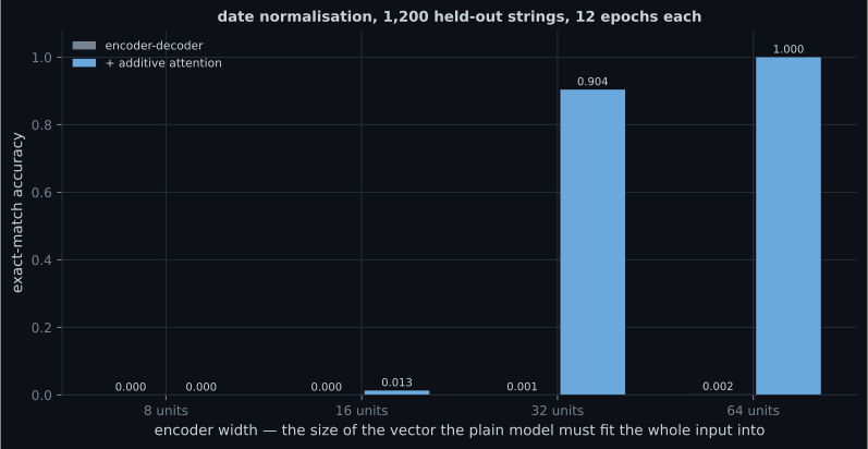
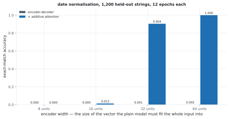
Encoder width	Plain, exact	Attention, exact	Plain, per character	Attention, per character
8	0.0000	0.0000	0.1432	0.4995
16	0.0000	0.0133	0.5524	0.7450
32	0.0008	0.9042	0.6467	0.9871
64	0.0017	1.0000	0.7277	1.0000

Exact match is a harsh metric on a ten-character output — one wrong digit fails the whole string — so the per-character columns are there to show that the plain model is not producing noise. At 64 units it gets 72.77% of output characters right while getting essentially no complete date right.

What the bottleneck actually drops

That combination — most characters right, almost no strings right — is only interesting if you look at which characters:

figure Both models at 64 units, 1,200 held-out strings matplotlib

The plain model's 0.7277 is not spread evenly at all. It has perfectly learned the two dashes (they are in the same place every time) and the year, which appears last in every input format and is therefore freshest in the final state. It then degrades along exactly the axis the bottleneck predicts: month first digit 0.7467, month second digit 0.1108, day first digit 0.3658, day second digit 0.0908.

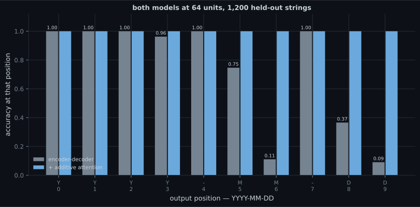
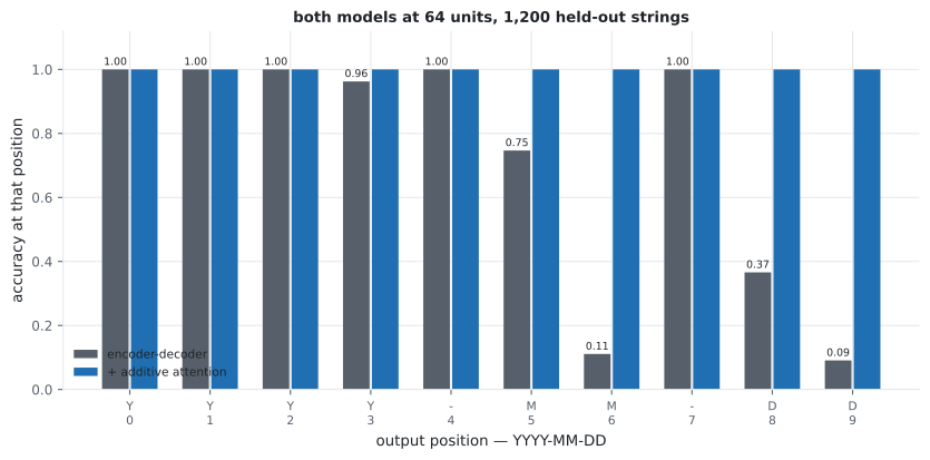
Output position	Plain	Attention
Y Y Y	1.0000	1.0000
Y (4th)	0.9625	1.0000
- (both)	1.0000	1.0000
M (1st)	0.7467	1.0000
M (2nd)	0.1108	1.0000
D (1st)	0.3658	1.0000
D (2nd)	0.0908	1.0000

Read the plain column as a memory decay curve. The dashes are free — they are at fixed positions and need no input at all. The year is perfect because it appears last in every one of the six input formats, so it is the most recent thing the encoder saw. The month is partially recoverable. The day, which appears earliest, is almost gone: 0.0908 on its second digit is close to the 0.10 you get by guessing a digit uniformly.

Bucketing by length showed nothing

The obvious experiment is to bucket by input length, on the theory that longer inputs overflow the state further. It was run: the plain model scored 0.7300, 0.7211, 0.7386 and 0.7086 across four length buckets — a spread of 0.0300, with no trend. Input length is not the axis that matters here; distance from the end of the input is. The figure above replaced the length figure for that reason.

Additive attention

The fix is to stop discarding the encoder’s intermediate states. Keep all of them — $\mathbf{h}_1 \dots \mathbf{h}_T$ — and let the decoder build a fresh summary at every output step, weighted toward whichever inputs are relevant right now.

At decoder step $t$, with previous decoder state $\mathbf{s}_{t-1}$:

$$e_{tj} = \mathbf{v}^\top \tanh\!\left(\mathbf{W}_{\!e}\,\mathbf{h}_j + \mathbf{W}_{\!d}\,\mathbf{s}_{t-1}\right)$$ $$\alpha_{tj} = \frac{\exp(e_{tj})}{\sum_{k=1}^{T} \exp(e_{tk})}, \qquad \mathbf{c}_t = \sum_{j=1}^{T} \alpha_{tj}\,\mathbf{h}_j$$

Three pieces, and each earns its place:

• $\mathbf{W}_{\!e}\mathbf{h}_j + \mathbf{W}_{\!d}\mathbf{s}_{t-1}$ — the additive part, and the reason for the name. Query and key are projected and summed, then squashed. Scaled dot-product attention replaces this whole expression with $\mathbf{q}^\top\mathbf{k}/\sqrt{d_k}$, which has no parameters and is one matrix multiply.
• The softmax makes the weights a distribution — they sum to 1 across input positions, so the context vector is a weighted average of real encoder states rather than an arbitrary combination.
• $\mathbf{c}_t$ is recomputed every step. That is the whole difference from the plain model, which computes its summary once.

The context vector is then concatenated with the embedded previous output token and fed to the decoder cell:

python

query = self.state_projection(state)[:, None, :]      # W_d s_{t-1}
scores = self.score(tf.nn.tanh(projected + query))[..., 0]
alpha = tf.nn.softmax(scores, axis=1)                 # over input positions
context = tf.reduce_sum(alpha[..., None] * encoded, axis=1)
cell_input = tf.concat([embedded[:, step, :], context], axis=-1)
output, [state] = self.cell(cell_input, [state])

At 64 units this costs 20,544 extra parameters (36,893 → 57,437) and roughly double the wall clock, 43.6 s → 83.5 s. It buys exact-match accuracy of 1.0000 against 0.0017.

diagram Diagram mermaid

  flowchart TD
  X["input characters"] --> E["GRU encoder"]
  E --> H["h_1 ... h_T
one state per input character"]
  H -->|"plain: keep only h_T"| B["64 numbers
for the whole input"]
  B --> D1["decoder
year 1.0000, day 0.0908"]
  H -->|"attention: keep all of them"| S["score each h_j
against s_(t-1)"]
  S --> A["softmax -> alpha_t"]
  A --> C["context c_t = sum alpha_tj h_j"]
  C --> D2["decoder
every position 1.0000"]

Reading the alignment

Attention produces a weight for every (output position, input position) pair, which plots as a matrix. This is the part that gets over-interpreted, so the task was chosen so the correct answer is known before looking.

figure One decoded example, weights taken from the trained model matplotlib

The output is 1977-09-19 and the input is 'wednesday 19 september 1977'. The year digits peak at input position 25 — inside '1977'. The month digit 9 peaks at position 15, which is inside 'september'. The day digits peak at position 11, which is the '9' of '19'. The model is not reading left to right; it jumps to whichever span of the input it needs.

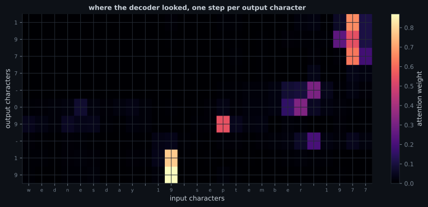
The measured peaks, character by character:

Output	Peak input position	Character there
1 9 7	25	7 (inside 1977)
7	22	space before 1977
-	22	space
0	21	r (end of september)
9	15	p (inside september)
-	22	space
1 9	11	9 (inside 19)

The three groups land on the three spans that carry the answer, and they land out of order — the year first, then the month word, then the day. That is what “the decoder chooses where to look” means concretely.

An alignment map is not an explanation

It is very easy to look at a heat map and narrate a story. Two guards make it evidence instead. First, know the right answer in advance — here the alignment is determined by the task, so a wrong map would be visible. Second, notice that the year digits peak on a space and the month digit on the letter p. The model is attending to positions whose encoder states are informative, not to the characters a human would point at. Encoder states are contextual; position 22’s state has already absorbed the year that follows it.

What the transformer kept and what it changed

Every piece of this mechanism survives into the transformer, with two substitutions.

Bahdanau, 2014	Transformer, 2017
score = $\mathbf{v}^\top\tanh(\mathbf{W}_{\!e}\mathbf{h} + \mathbf{W}_{\!d}\mathbf{s})$	score = $\mathbf{q}^\top\mathbf{k}/\sqrt{d_k}$
query is the decoder’s recurrent state	query is a projection of a token, no recurrence
one attention head	many heads in parallel
encoder is a GRU, so steps are sequential	encoder is attention, so steps are parallel
context concatenated into the recurrent cell	context is the residual stream itself

The important change is the second row. Bahdanau’s query comes from a recurrent state, so the decoder still runs one step at a time and the encoder still walks the input sequentially. Removing recurrence — replacing the query source with a projection of the token itself — is what makes the whole sequence computable in parallel, and that is the transformer’s actual contribution. The scoring function got simpler along the way, but that was a bonus, not the point.

sketch Where the decoder looks p5.js Pause Restart

Click an output character. The bars show the measured attention weight peak for that character over the input string - the three groups land on three different spans.

sketch The measured table, ranked p5.js Pause Restart

Click a column to rank every row by it. The bars are that column's values and the highest and lowest are computed from the numbers, not written in.

Pitfalls

• Concluding “attention beats recurrence”. Attention here is added to a recurrent encoder–decoder. Both models are recurrent; only one has a bottleneck.
• Reading exact match alone. 0.0017 against 1.0000 suggests the plain model learned nothing. Per character it reached 0.7277, and the per-position split is where the actual finding is.
• Assuming longer inputs are the problem. Measured spread across length buckets: 0.0300, no trend. Distance from the end of the input is the axis that matters.
• Narrating an alignment map without knowing the answer. The year digits peak on a space. Encoder states are contextual, so the bright cell is not always where a human would point.
• Forgetting the cost. 20,544 extra parameters and 1.9× the wall clock, and the context vector is recomputed at every output step, so attention costs $O(T_{\text{in}} \times T_{\text{out}})$ score evaluations where the bottleneck costs a constant number.
• Comparing at one encoder width. At 8 units both models score 0.0000 exact. A single-width comparison could have shown attention making no difference at all.

Recap

• A plain encoder–decoder passes the entire input through one fixed-size vector; at 64 units that is 64 numbers for a 27-character string.
• On date normalisation the plain model reached 0.0017 exact match against attention’s 1.0000, and per character 0.7277 against 1.0000.
• The per-position split shows what the bottleneck drops: year and separators 1.0000, day second digit 0.0908 — the failure tracks distance from the end of the input, not input length (spread across length buckets: 0.0300).
• Additive attention scores every encoder state against the previous decoder state, softmaxes, and averages — one context vector per output step instead of one per sequence.
• The measured alignment jumps between three spans out of order, and peaks on positions whose states are informative rather than on the characters a human would choose.
• The transformer keeps the score-softmax-average structure and replaces the recurrent query with a token projection, which is what removes the sequential dependency.

Next

Phase 5 takes the mechanism on this page, removes the recurrence around it, and asks what is left: Attention from Scratch (Queries, Keys and Values).

pch.quizTag pch.quizDefaultTitle

1. The plain encoder–decoder scored 1.0000 on all four year digits and 0.0908 on the day's second digit. What explains the pattern?

   A Year digits are easier to predict than day digits B The year appears last in every input format, so it is the most recent thing the fixed-size final state absorbed; the day appears earliest and has been overwritten C The model was only trained on years D Day digits have higher entropy
   pch.quizShowAnswer

   B — The year appears last in every input format, so it is the most recent thing the fixed-size final state absorbed; the day appears earliest and has been overwritten

2. Bucketing the same results by input length gave 0.7300, 0.7211, 0.7386 and 0.7086 — a spread of 0.0300 with no trend. Why report a null result?

   A To fill space B Because it rules out the obvious explanation: the bottleneck is not about how long the input is but about how far the needed information sits from its end C Because the buckets were too small D Because length always matters eventually
   pch.quizShowAnswer

   B — Because it rules out the obvious explanation: the bottleneck is not about how long the input is but about how far the needed information sits from its end

3. In additive attention, what makes the mechanism 'additive'?

   A The context vector is added to the decoder output B The encoder and decoder projections are summed inside a tanh before scoring — W_e h + W_d s — rather than multiplied as a dot product C The attention weights add up to one D Multiple heads are added together
   pch.quizShowAnswer

   B — The encoder and decoder projections are summed inside a tanh before scoring — W_e h + W_d s — rather than multiplied as a dot product

4. For the input 'wednesday 19 september 1977', the year digits peaked at input position 22 and 25 — one of which is a space. Is the alignment wrong?

   A Yes, it should peak on the digits themselves B No — the model attends to encoder STATES, and a GRU state at position 22 has already absorbed the characters around it, so it can be the most informative place to look C Yes, the model is guessing D No, spaces are the most important token
   pch.quizShowAnswer

   B — No — the model attends to encoder STATES, and a GRU state at position 22 has already absorbed the characters around it, so it can be the most informative place to look

5. What did the transformer actually change relative to this mechanism?

   A It introduced attention B It replaced the recurrent decoder state as the query source with a projection of the token itself, which removes the sequential dependency and lets the whole sequence be computed in parallel C It made attention weights sum to one D It removed the softmax
   pch.quizShowAnswer

   B — It replaced the recurrent decoder state as the query source with a projection of the token itself, which removes the sequential dependency and lets the whole sequence be computed in parallel

6. At 8 encoder units both models scored 0.0000 exact match. What would a single-width comparison have concluded?

   A The correct thing — both models are equivalent B That attention makes no difference, which the 32- and 64-unit columns refute (0.9042 and 1.0000 against 0.0008 and 0.0017) C That the task is impossible D That 8 units is the right width
   pch.quizShowAnswer

   B — That attention makes no difference, which the 32- and 64-unit columns refute (0.9042 and 1.0000 against 0.0008 and 0.0017)

🧪 Try It Yourself

pch.exerciseTag pch.exerciseTitle

pch.exerciseTag pch.exerciseTitle

pch.exerciseTag pch.exerciseTitle

pch.exerciseTag pch.exerciseTitle

pch.exerciseTag pch.exerciseTitle

pch.exerciseTag pch.exerciseTitle