What you’ll learn

• agglomerative clustering as a sequence of $n - 1$ merges, traced in full on eight points
• the four linkage rules, each computed by hand from the same distance matrix
• how to read a dendrogram, and why the vertical axis is the only part that carries information
• the Lance-Williams recurrence that makes all four rules one algorithm
• the measured single-versus-Ward trade-off: ARI 1.00 / 0.00 against 0.13 / 0.93
• how to choose a cut height without committing to $k$ in advance
• the cophenetic correlation, and why $O(n^2)$ memory ends the party around 30,000 rows

Intuition

k-means asks you for $k$ before it will tell you anything. Hierarchical clustering refuses to commit. It builds every clustering at once — from $n$ singleton clusters down to one cluster containing everything — and hands you the whole nested family as a tree. You pick where to cut afterwards, having seen the structure.

The agglomerative (bottom-up) version is a loop of exactly three lines:

1. Start with every point as its own cluster.
2. Merge the two closest clusters.
3. Repeat until one cluster remains.

The only difficulty is step 2, because “closest” between two sets of points is not defined by the distance between two points. That definition is the linkage rule, and it is the entire character of the algorithm.

  flowchart TD
  A["n singleton clusters"] --> B["Compute all pairwise cluster distances
using the linkage rule"]
  B --> C["Merge the closest pair"]
  C --> D["Record the merge height in the dendrogram"]
  D --> E{"One cluster left?"}
  E -->|"no"| B
  E -->|"yes"| F["Full tree.
Cut it wherever you like."]

There is also a divisive (top-down) version that starts with one cluster and splits recursively. It is rarely used — the first split alone is a $2^{n-1}$ search — so “hierarchical clustering” in practice means agglomerative.

The math

Let $A$ and $B$ be two clusters and $d(\cdot, \cdot)$ the point-level distance. The four standard linkage rules define the cluster-level distance $D(A, B)$:

Single linkage — the nearest pair:

Complete linkage — the furthest pair:

Average linkage — the mean over all pairs:

Ward linkage minimises the increase in within-cluster sum of squares caused by the merge. That increase has a closed form:

where $\bar{\mathbf{a}}$ and $\bar{\mathbf{b}}$ are the two centroids. SciPy reports the merge height as $\sqrt{2\Delta}$, so the plotted Ward distance is

Ward is the direct hierarchical analogue of k-means: both minimise within-cluster sum of squares, one greedily bottom-up and one by alternating optimisation. Ward requires Euclidean distance; the other three accept any metric.

One recurrence, four rules

Naively, every merge would require recomputing distances from scratch. The Lance-Williams recurrence avoids that. After merging $A$ and $B$ into $A \cup B$, the distance to any other cluster $C$ is:

Writing $n_A$, $n_B$ and $n_C$ for the three cluster sizes, and $n_T = n_A + n_B + n_C$:

Single and complete differ only in the sign of $\gamma$ — half the difference, added or subtracted. That one sign is the difference between chaining and compactness.

Worked example by hand

Eight points, labelled A through H:

The Euclidean distance matrix, rounded to three decimals:

Merge 1. The smallest off-diagonal entry is $d(A, B) = 0.5385$. Merge them into $\{A, B\}$.

Now the linkage rules diverge. The new cluster $\{A, B\}$ needs a distance to C. From the matrix, $d(A, C) = 1.0198$ and $d(B, C) = 0.8544$, so:

For the Ward figure: $\overline{AB} = (1.25,\ 1.10)$ and $C = (1.2,\ 2.0)$, so the centroid gap is $\sqrt{0.05^2 + 0.9^2} = 0.9014$, and $\sqrt{4/3} \times 0.9014 = 1.0408$.

Every one of these matches SciPy exactly.

Merges 2 and 3 are the same under all four rules, because both involve singletons: $d(D, E) = 0.7211$ and $d(G, H) = 0.7211$.

Here is the complete Ward trace:

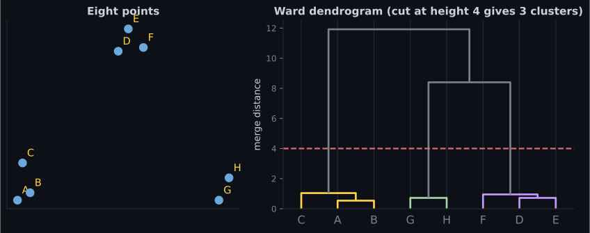
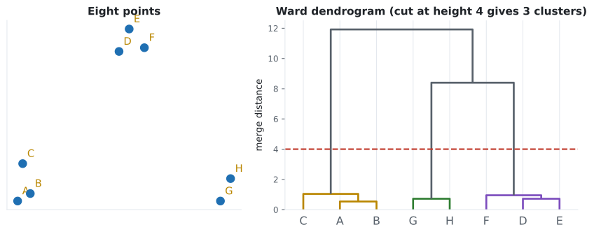
Notice the gap. The first five merges all happen below height 1.05; the sixth jumps to 8.40. That jump is the signal, and cutting anywhere between 1.05 and 8.40 gives three clusters: $\{A, B, C\}$, $\{D, E, F\}$, $\{G, H\}$ — exactly the three visual groups.

figureEight points and their Ward treematplotlib

Reading a dendrogram

Three rules cover almost every mistake people make with these plots.

The vertical axis is the only quantitative axis. Height means merge distance. Read it.

Horizontal position is arbitrary. At each merge, either subtree can be drawn on the left. The same tree has $2^{n-1}$ valid drawings. Two leaves being drawn side by side means nothing unless they are joined by a low bar.

A cut is a horizontal line. The number of vertical branches it crosses is the number of clusters you get. Cut low for many small clusters, high for few large ones.

The long vertical runs are the interesting part. A branch that survives a long height interval without merging is a cluster that stayed distinct across a wide range of thresholds — evidence of real separation.

See it move

The next sketch is the one that matters: the same eight points under all four linkage rules, with the merge order and heights recomputed for each.

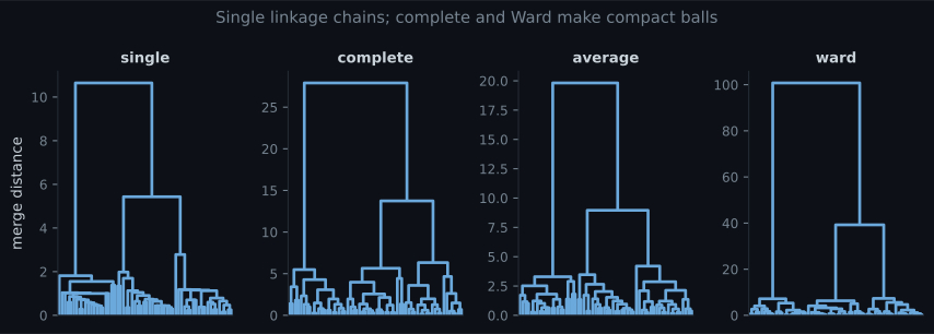
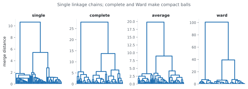
Watch the tallest merge as you cycle: 4.879 for single, 8.421 for complete, 6.632 for average, 11.922 for Ward. The tree’s shape changes; the data never does.

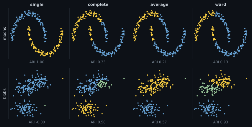
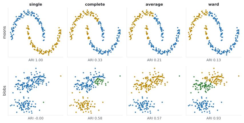
The linkage trade-off, measured

The four rules are not four flavours of the same thing. They encode genuinely different beliefs about what a cluster is, and the consequences are stark.

figureThe same four rules on two datasetsmatplotlib

Single linkage’s failure on blobs is worth understanding. It merges whenever any two points are close, so a thin trail of points between two blobs is enough to fuse them — the chaining effect. On the moons, chaining is exactly right: each moon is a connected dense path. On blobs with a few scattered points, chaining swallows everything.

figureFour rules, four trees, one datasetmatplotlib

Choosing where to cut

Two approaches, and they answer different questions.

By $k$. Pass n_clusters=4n_clusters=4 and let the algorithm cut wherever it must. Use this when the number is fixed by something external.

By height. Pass a distance_thresholddistance_threshold and let the number of clusters fall out. Use this when you want the data to decide.

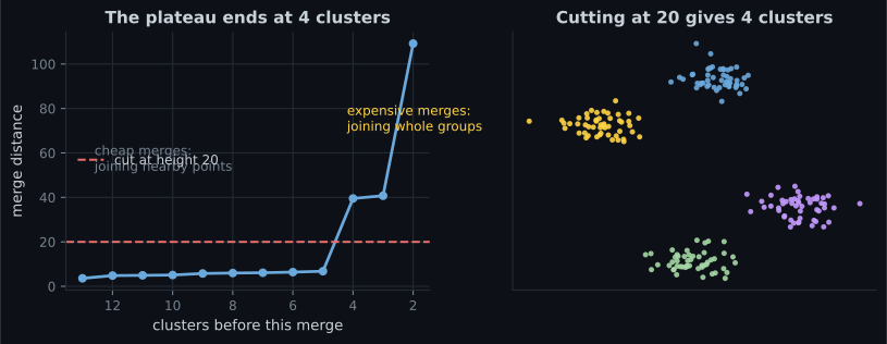
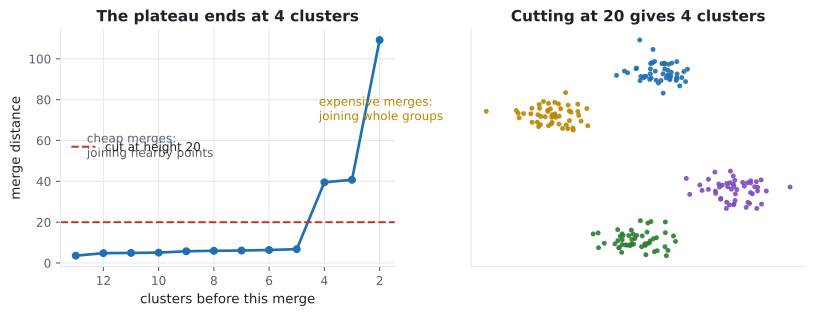
To pick a height, plot the merge distances and find where they stop being cheap. On 200 points containing 4 blobs, the last eight Ward merges are at heights:

Five merges under 7, then a jump to 39.5. Anything between about 7 and 39 gives the same answer, and cutting at 20 returns exactly 4 clusters.

figureWhere the merges stop being cheapmatplotlib

Cophenetic correlation

How faithfully does the tree represent the original distances? The cophenetic distance between two points is the height at which they first end up in the same cluster. Correlate those with the original pairwise distances:

On the eight-point example: single 0.9238, complete 0.9311, average 0.9398, Ward 0.9338. Average linkage wins, which is not a coincidence — average linkage optimises something close to this quantity directly. Values above about 0.75 mean the tree is a reasonable summary; well below that, the dendrogram is distorting the geometry and you should not read structure into it.

In code

import numpy as np
from sklearn.cluster import AgglomerativeClustering
 
X = np.array([[1.0, 1.0], [1.5, 1.2], [1.2, 2.0], [5.0, 5.0],
              [5.4, 5.6], [6.0, 5.1], [9.0, 1.0], [9.4, 1.6]])
 
# Option A: I know how many clusters I want.
by_k = AgglomerativeClustering(n_clusters=3, linkage="ward").fit(X)
print(by_k.labels_)                       # [0 0 0 1 1 1 2 2]
 
# Option B: I know how far apart clusters must be. n_clusters must be None.
by_height = AgglomerativeClustering(
    n_clusters=None, distance_threshold=4.0, linkage="ward"
).fit(X)
print(by_height.n_clusters_)              # 3
 
# compute_distances=True populates .distances_ so you can plot the tree
tree = AgglomerativeClustering(n_clusters=3, compute_distances=True).fit(X)
print(tree.distances_.round(4))           # [0.5385 0.7211 0.7211 0.9522 1.0408 8.4013 11.922]

import numpy as np
from sklearn.cluster import AgglomerativeClustering
 
X = np.array([[1.0, 1.0], [1.5, 1.2], [1.2, 2.0], [5.0, 5.0],
              [5.4, 5.6], [6.0, 5.1], [9.0, 1.0], [9.4, 1.6]])
 
# Option A: I know how many clusters I want.
by_k = AgglomerativeClustering(n_clusters=3, linkage="ward").fit(X)
print(by_k.labels_)                       # [0 0 0 1 1 1 2 2]
 
# Option B: I know how far apart clusters must be. n_clusters must be None.
by_height = AgglomerativeClustering(
    n_clusters=None, distance_threshold=4.0, linkage="ward"
).fit(X)
print(by_height.n_clusters_)              # 3
 
# compute_distances=True populates .distances_ so you can plot the tree
tree = AgglomerativeClustering(n_clusters=3, compute_distances=True).fit(X)
print(tree.distances_.round(4))           # [0.5385 0.7211 0.7211 0.9522 1.0408 8.4013 11.922]

For the dendrogram itself, go to SciPy — scikit-learn does not plot one.

import matplotlib.pyplot as plt
import numpy as np
from scipy.cluster.hierarchy import cophenet, dendrogram, fcluster, linkage
from scipy.spatial.distance import pdist
 
X = np.array([[1.0, 1.0], [1.5, 1.2], [1.2, 2.0], [5.0, 5.0],
              [5.4, 5.6], [6.0, 5.1], [9.0, 1.0], [9.4, 1.6]])
labels = list("ABCDEFGH")
 
Z = linkage(X, method="ward")
# Z has one row per merge: [left_id, right_id, height, size_of_new_cluster]
print(Z.round(4))
 
print("cophenetic correlation", round(cophenet(Z, pdist(X))[0], 4))   # 0.9338
print("cut at 4.0 ->", fcluster(Z, t=4.0, criterion="distance"))      # [1 1 1 3 3 3 2 2]
print("exactly 3  ->", fcluster(Z, t=3, criterion="maxclust"))        # [1 1 1 3 3 3 2 2]
 
dendrogram(Z, labels=labels)
plt.axhline(4.0, color="red", linestyle="--")
plt.ylabel("merge distance")
plt.show()

import matplotlib.pyplot as plt
import numpy as np
from scipy.cluster.hierarchy import cophenet, dendrogram, fcluster, linkage
from scipy.spatial.distance import pdist
 
X = np.array([[1.0, 1.0], [1.5, 1.2], [1.2, 2.0], [5.0, 5.0],
              [5.4, 5.6], [6.0, 5.1], [9.0, 1.0], [9.4, 1.6]])
labels = list("ABCDEFGH")
 
Z = linkage(X, method="ward")
# Z has one row per merge: [left_id, right_id, height, size_of_new_cluster]
print(Z.round(4))
 
print("cophenetic correlation", round(cophenet(Z, pdist(X))[0], 4))   # 0.9338
print("cut at 4.0 ->", fcluster(Z, t=4.0, criterion="distance"))      # [1 1 1 3 3 3 2 2]
print("exactly 3  ->", fcluster(Z, t=3, criterion="maxclust"))        # [1 1 1 3 3 3 2 2]
 
dendrogram(Z, labels=labels)
plt.axhline(4.0, color="red", linestyle="--")
plt.ylabel("merge distance")
plt.show()

linkagelinkage accepts either a raw data matrix or a condensed distance vector from pdistpdist, which is how you use a custom metric:

from scipy.cluster.hierarchy import linkage
from scipy.spatial.distance import pdist
 
# Cosine distance for text; note that ward would reject this — it needs Euclidean.
Z = linkage(pdist(X_tfidf, metric="cosine"), method="average")

from scipy.cluster.hierarchy import linkage
from scipy.spatial.distance import pdist
 
# Cosine distance for text; note that ward would reject this — it needs Euclidean.
Z = linkage(pdist(X_tfidf, metric="cosine"), method="average")

Connectivity constraints

If you already know which points could plausibly belong together — pixels that touch, cities joined by a road, samples adjacent in time — pass a connectivity matrix. Merges are then only considered between connected clusters, which both encodes the domain knowledge and drops the cost substantially.

from sklearn.cluster import AgglomerativeClustering
from sklearn.neighbors import kneighbors_graph
 
# Only allow merges between points that are among each other's 10 nearest neighbours.
conn = kneighbors_graph(X, n_neighbors=10, include_self=False)
model = AgglomerativeClustering(n_clusters=4, connectivity=conn, linkage="ward").fit(X)

from sklearn.cluster import AgglomerativeClustering
from sklearn.neighbors import kneighbors_graph
 
# Only allow merges between points that are among each other's 10 nearest neighbours.
conn = kneighbors_graph(X, n_neighbors=10, include_self=False)
model = AgglomerativeClustering(n_clusters=4, connectivity=conn, linkage="ward").fit(X)

Without a connectivity constraint, Ward on $n$ points needs the full $O(n^2)$ distance structure. At 30,000 rows that is around 900 million float64 entries, roughly 7 GB — the practical ceiling for this algorithm on a laptop.

Pitfalls

Reading meaning into left-right order. Any subtree can be flipped. Adjacent leaves are not necessarily similar; only a low joining bar means similar.

Using Ward with a non-Euclidean metric. scikit-learn raises an error; SciPy quietly computes something meaningless. Ward’s derivation is entirely about sums of squares.

Forgetting merges are permanent. Agglomerative clustering never reconsiders. One bad early merge, caused by a single outlier bridging two groups, propagates all the way up. k-means can recover from a bad start over iterations; this cannot.

Hitting the memory wall by surprise. The $O(n^2)$ distance structure is fine at 5,000 rows and fatal at 50,000. Add a connectivityconnectivity graph, sample, or switch to DBSCAN.

Choosing single linkage without seeing the data. It is either the best rule available (ARI 1.00 on moons) or catastrophic (ARI 0.00 on blobs). Plot the dendrogram: a lopsided comb with no clear tall split means chaining has already happened.

Expecting predictpredict. There is no such method. The cluster definitions are relative to the training set, so labelling a new point means refitting or, pragmatically, assigning it to the nearest cluster centroid yourself.

Not scaling. Same as everywhere: distances drive every merge.

Compare

🧪 Try It Yourself

Exercise 1 – Four linkages, one pair of clusters

Exercise 2 – Read the linkage matrix

Exercise 3 – Cut by height instead of by k

Exercise 4 – The chaining trade-off, measured

Exercise 5 – Which tree is most faithful?

Recap

• Agglomerative clustering performs $n - 1$ merges and hands you every clustering at once; you cut afterwards.
• The linkage rule defines set-to-set distance. On one pair from the worked matrix: single 0.8544, complete 1.0198, average 0.9371, Ward 1.0408.
• All four are instances of the Lance-Williams recurrence; single and complete differ only in the sign of $\gamma$.
• Ward’s tree on the eight points jumps from 1.04 to 8.40 at merge 6 — that gap is the three real groups.
• The trade-off is real and measured: single linkage scores 1.00 on moons and 0.00 on blobs; Ward scores 0.13 and 0.93.
• Cut by distance_thresholddistance_threshold when you want the data to decide $k$; look for the plateau in the merge heights.
• Cophenetic correlation says how faithful the tree is — average linkage won at 0.9398 here.
• $O(n^2)$ memory is the binding constraint: about 30,000 rows without a connectivity graph.

Exercise 6 – The linkage decides what a cluster is

Next

DBSCAN - Density-Based Clustering — an algorithm that needs no $k$ at all, finds arbitrarily shaped clusters, and is the only method in this phase that can say “this point belongs to nothing”.