Multiple Linear Regression

What you’ll learn

• the matrix form of the model, and how to derive the Normal Equation by setting a gradient to zero
• how to solve a three-parameter fit by hand when the design is orthogonal
• the exact meaning of “holding all other features constant”, and when that phrase is a lie
• why coefficients are only comparable after standardising
• what multicollinearity breaks — and, just as importantly, what it does not
• why scikit-learn uses lstsq rather than inverting a matrix

Intuition

One feature gives you a line. Two features give you a plane. Ten features give you a hyperplane nobody can picture — but the arithmetic never changes: multiply each feature by its weight, add them all up, add the bias.

What does change is interpretation. With one feature, the slope is simply “how $y$ moves with $x$”. With several correlated features, each coefficient answers a much narrower question: how $y$ moves with this feature once the others have already had their say. Miss that and you will misread almost every model you fit.

diagram Diagram mermaid

  flowchart LR
  X1["x1  size"] --> M["Weighted sum
theta transpose x"]
  X2["x2  bedrooms"] --> M
  X3["x3  age"] --> M
  XN["x_n  ..."] --> M
  M --> Y["Prediction ŷ"]

The math

The model in matrix form

Stack $m$ instances as rows of a design matrix $\mathbf{X} \in \mathbb{R}^{m\times(n+1)}$, whose first column is all ones:

$$\hat{\mathbf{y}} = \mathbf{X}\boldsymbol{\theta}, \qquad J(\boldsymbol{\theta}) = \frac{1}{m}\lVert \mathbf{X}\boldsymbol{\theta} - \mathbf{y}\rVert_2^2$$

Deriving the Normal Equation

Expand the squared norm as an inner product and drop the constant $1/m$ — it cannot move the minimiser:

$$J(\boldsymbol{\theta}) \propto (\mathbf{X}\boldsymbol{\theta} - \mathbf{y})^\top(\mathbf{X}\boldsymbol{\theta} - \mathbf{y}) = \boldsymbol{\theta}^\top\mathbf{X}^\top\mathbf{X}\boldsymbol{\theta} - 2\boldsymbol{\theta}^\top\mathbf{X}^\top\mathbf{y} + \mathbf{y}^\top\mathbf{y}$$

Differentiate with respect to $\boldsymbol{\theta}$ using two standard identities — $\nabla_{\boldsymbol{\theta}}(\boldsymbol{\theta}^\top\mathbf{A}\boldsymbol{\theta}) = 2\mathbf{A}\boldsymbol{\theta}$ for symmetric $\mathbf{A}$, and $\nabla_{\boldsymbol{\theta}}(\boldsymbol{\theta}^\top\mathbf{b}) = \mathbf{b}$:

$$\nabla_{\boldsymbol{\theta}} J = 2\mathbf{X}^\top\mathbf{X}\boldsymbol{\theta} - 2\mathbf{X}^\top\mathbf{y} = \mathbf{0}$$ $$\boxed{\;\boldsymbol{\theta} = (\mathbf{X}^\top\mathbf{X})^{-1}\mathbf{X}^\top\mathbf{y}\;}$$

That is the Normal Equation: one formula, no iteration, no learning rate.

Where this comes from

Those two gradient identities are derived in Useful Identities for Computing Gradients. Geometrically, $\mathbf{X}(\mathbf{X}^\top\mathbf{X})^{-1}\mathbf{X}^\top$ projects onto the column space of $\mathbf{X}$ — least squares is the orthogonal projection of $\mathbf{y}$ onto the space of predictions the model can actually produce.

The residual is orthogonal to every feature

Rearranged, the Normal Equation says $\mathbf{X}^\top(\mathbf{y} - \mathbf{X}\boldsymbol{\theta}) = \mathbf{0}$: the residual vector is perpendicular to every column of $\mathbf{X}$. Two consequences you can check on any fit:

• because the first column is all ones, the residuals sum to zero
• because every other column is a feature, the residuals are uncorrelated with each feature

If either fails, you did not fit least squares.

Worked example by hand

An orthogonal design — a small experiment where two on/off factors were varied deliberately. Both are coded $-1$ (off) and $+1$ (on), which keeps the arithmetic exact.

$i$	$x_0$	promotion $x_1$	weekend $x_2$	sales $y$
1	1	−1	−1	1
2	1	−1	+1	3
3	1	+1	−1	5
4	1	+1	+1	8

Step 1 — build $\mathbf{X}^\top\mathbf{X}$. Every column holds four entries of $\pm 1$, and any two different columns are orthogonal, so all off-diagonal entries vanish:

$$\mathbf{X}^\top\mathbf{X} = \begin{bmatrix} 4 & 0 & 0 \\ 0 & 4 & 0 \\ 0 & 0 & 4 \end{bmatrix}, \qquad (\mathbf{X}^\top\mathbf{X})^{-1} = \tfrac{1}{4}\mathbf{I}$$

Step 2 — build $\mathbf{X}^\top\mathbf{y}$.

$$\mathbf{X}^\top\mathbf{y} = \begin{bmatrix} 1+3+5+8 \\ -1-3+5+8 \\ -1+3-5+8 \end{bmatrix} = \begin{bmatrix} 17 \\ 9 \\ 5 \end{bmatrix}$$

Step 3 — multiply.

$$\boldsymbol{\theta} = \tfrac{1}{4}\begin{bmatrix} 17 \\ 9 \\ 5 \end{bmatrix} = \begin{bmatrix} 4.25 \\ 2.25 \\ 1.25 \end{bmatrix}$$

So $\hat{y} = 4.25 + 2.25\,x_1 + 1.25\,x_2$.

Step 4 — check the fit.

$i$	$x_1$	$x_2$	$\hat{y}$	$y$	residual
1	−1	−1	0.75	1	+0.25
2	−1	+1	3.25	3	−0.25
3	+1	−1	5.25	5	−0.25
4	+1	+1	7.75	8	+0.25
					0.00

$$\text{SSE} = 4(0.25)^2 = 0.25, \qquad \text{SST} = 26.75, \qquad R^2 = 1 - \frac{0.25}{26.75} \approx 0.991$$

Residuals sum to zero, and they are orthogonal to both feature columns — $\sum x_1 e = -0.25 + 0.25 - 0.25 + 0.25 = 0$, and the same for $x_2$. Exactly what the Normal Equation promised.

Reading the coefficients. Because the features are coded $\pm 1$, switching the promotion on moves sales by $2 \times 2.25 = 4.5$ units, and a weekend adds $2 \times 1.25 = 2.5$. The promotion is the stronger lever, and here that comparison is legitimate — both features share a scale and are uncorrelated.

See it move

The Normal Equation solves for the plane in one shot. Below, a flat baseline plane tilts into the least-squares fit over two features; the red stems are residuals shrinking as it locks in.

sketch Fitting a plane with two features p5.js Pause Restart

The Normal Equation tilts a flat baseline plane into the least-squares fit over two features; residual stems shrink as it locks in.

From scratch

Three ways to solve the same system, in increasing order of how much you should trust them:

normal_equation.py

import numpy as np
 
X = np.array([[1, -1, -1],
              [1, -1,  1],
              [1,  1, -1],
              [1,  1,  1]], dtype=float)
y = np.array([1.0, 3.0, 5.0, 8.0])
 
# 1. Textbook form — never use this in production
theta_inv = np.linalg.inv(X.T @ X) @ X.T @ y
 
# 2. Solve the linear system instead of inverting: faster, better conditioned
theta_solve = np.linalg.solve(X.T @ X, X.T @ y)
 
# 3. What scikit-learn actually does: least squares via SVD.
#    Still returns an answer when X.T @ X is singular.
theta_lstsq, *_ = np.linalg.lstsq(X, y, rcond=None)
 
print(theta_inv.round(4))     # [4.25 2.25 1.25]
print(theta_solve.round(4))   # [4.25 2.25 1.25]
print(theta_lstsq.round(4))   # [4.25 2.25 1.25]
 
resid = y - X @ theta_lstsq
print(resid.round(4))                 # [ 0.25 -0.25 -0.25  0.25]
print(round(resid.sum(), 10))         # 0.0
print((X.T @ resid).round(10))        # [0. 0. 0.]  <- orthogonal to every column

Never call np.linalg.inv on X.T @ X

Explicit inversion is slower and numerically worse than solving the system, and it fails outright when features are perfectly collinear. lstsq uses the SVD-based pseudoinverse, which returns the minimum-norm solution instead of raising. That is precisely why LinearRegression never errors on duplicate columns — it quietly splits the weight between them.

With scikit-learn

diabetes_multi.py

from sklearn.datasets import load_diabetes
from sklearn.linear_model import LinearRegression
from sklearn.model_selection import train_test_split
from sklearn.metrics import mean_squared_error
 
data = load_diabetes()
X_train, X_test, y_train, y_test = train_test_split(
    data.data, data.target, test_size=0.3, random_state=42
)
 
model = LinearRegression().fit(X_train, y_train)
 
print(f"train R^2 = {model.score(X_train, y_train):.4f}")   # train R^2 = 0.5244
print(f"test  R^2 = {model.score(X_test, y_test):.4f}")     # test  R^2 = 0.4773
 
rmse = mean_squared_error(y_test, model.predict(X_test)) ** 0.5
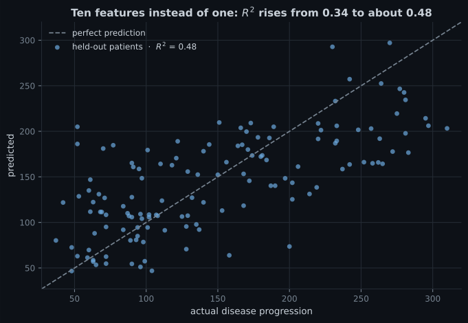
print(f"test RMSE = {rmse:.2f}")                            # test RMSE = 53.12

Ten features lift test $R^2$ from the 0.34 that BMI alone managed to 0.48. The gap between train (0.52) and test (0.48) is small, which is what a well-behaved linear model looks like.

figure Predicted against actual on held-out data matplotlib

The single most useful diagnostic once you pass two features. Points should hug the diagonal with no curvature and no fanning.

Reading the plot

• No systematic curve. Points sit around the diagonal rather than bowing above or below it, so a linear model is a reasonable shape here.
• Compression at the extremes. Low actual values are over-predicted and high ones under-predicted — the classic signature of a model that has captured the trend but not the tails.
• Vertical spread is the error. At any actual value the scatter is roughly ±50, which matches the RMSE of 53.

Interpreting coefficients

Raw coefficients are not comparable

A coefficient is expressed in target units per one unit of that feature. A coefficient of 949 on BMI and 3 on age says nothing about relative importance until both features share a scale. Standardise first, and each coefficient becomes “target change per one standard deviation”:

standardised_coefficients.py

from sklearn.datasets import load_diabetes
from sklearn.linear_model import LinearRegression
from sklearn.preprocessing import StandardScaler
 
data = load_diabetes()
X = StandardScaler().fit_transform(data.data)
model = LinearRegression().fit(X, data.target)
 
for name, coef in sorted(zip(data.feature_names, model.coef_),
                         key=lambda pair: -abs(pair[1])):
    print(f"{name:>5} {coef:8.2f}")
 
#    s1   -37.68
#    s5    35.73
#   bmi    24.73
#    s2    22.68
#    bp    15.43
#   sex   -11.41
#    s4     8.42
#    s3     4.81
#    s6     3.22
#   age    -0.48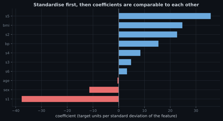

figure Standardised coefficients, sorted matplotlib

Now the bars are comparable. s1 and s5 dominate; age contributes essentially nothing once the other nine features are present.

“Holding everything else constant”

The textbook reading of $\theta_j$ is: the change in $\hat{y}$ for a one-unit increase in $x_j$, with all other features held fixed. That clause is doing enormous work. If two features always move together in the real world, no observation ever shows one changing while the other stays put — so the coefficient describes a scenario your data never contained.

That is why age scores −0.48 here despite age plainly mattering to disease progression: its information is already carried by blood pressure and the serum measurements. The coefficient does not say “age does not matter”, it says “age adds nothing beyond the other nine columns”.

Multicollinearity

figure 120 refits on fresh samples from the same process matplotlib

Correlated features do not bias the coefficients — the cloud is still centred on the truth — but they scatter them enormously. Any single fit could report almost anything.

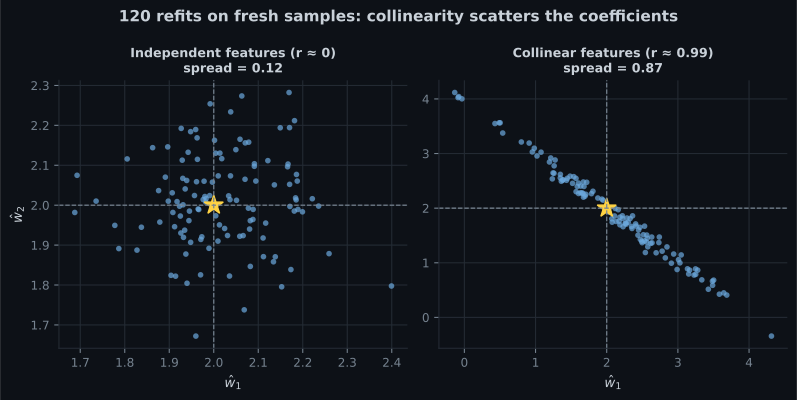
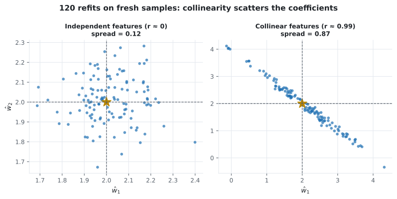
Detect it with the variance inflation factor. For feature $j$, regress it on all the others and take:

$$\text{VIF}_j = \frac{1}{1 - R^2_j}$$

A VIF of 1 means no collinearity, above 5 is worth a look, and above 10 means that coefficient is close to meaningless on its own.

vif.py

import numpy as np
from sklearn.datasets import load_diabetes
from sklearn.linear_model import LinearRegression
 
data = load_diabetes()
X = data.data
 
for j, name in enumerate(data.feature_names):
    others = np.delete(X, j, axis=1)
    r2 = LinearRegression().fit(others, X[:, j]).score(others, X[:, j])
    vif = 1 / (1 - r2)
    flag = "  <-- high" if vif > 10 else ""
    print(f"{name:>5}  VIF = {vif:7.2f}{flag}")
 
#   age  VIF =    1.22
#   sex  VIF =    1.28
#   bmi  VIF =    1.51
#    bp  VIF =    1.46
#    s1  VIF =   59.20  <-- high
#    s2  VIF =   39.19  <-- high
#    s3  VIF =   15.40  <-- high
#    s4  VIF =    8.89
#    s5  VIF =   10.08  <-- high
#    s6  VIF =    1.48

The serum measurements are heavily entangled, which is exactly why s1 and s5 carry large coefficients of opposite sign: the model is taking a difference between two nearly identical columns.

What collinearity does not break

Predictions. The fitted surface, the $R^2$ and the RMSE are all fine — the model simply cannot decide which of the correlated features deserves the credit. If you only need forecasts you can live with it. If you need to explain the model, you cannot. Ridge regression is the standard fix.

pch.algoTag Multiple Linear Regression (OLS) Supervised · Regression

pch.algoApi sklearn.linear_model.LinearRegression

pch.algoAssumes

• The target is linear in the parameters
• Observations are independent
• Residual variance is constant across the feature space
• No perfect collinearity among the features

pch.algoCost

pch.algoTrain

O(m·n² + n³)

pch.algoPredict

O(n)

pch.algoMemory

O(n)

m = samples, n = features; training cost is dominated by forming and factorising X transpose X

pch.algoHyperparams

• fit_intercept default True Leave on unless the data is already centred or theory forces a zero intercept.
• positive default False Constrain every coefficient to be non-negative — useful for mixing weights and physical quantities.
• n_jobs default None Parallelism for the multi-target case only; it will not speed up a single target.

pch.algoReachFor

• You want a strong, fast, interpretable baseline on tabular data
• The number of features is comfortably smaller than the number of samples
• You need coefficients you can put in a report

pch.algoLookElsewhere

• Features outnumber samples — the solution is not unique, so use Ridge or Lasso
• Features are heavily collinear and you need to interpret individual effects
• The relationship is strongly non-linear and you cannot engineer the terms
• Outliers dominate the target

Pitfalls

Adding features always improves training $R^2$

Every extra column can only reduce training error, even a column of pure noise. Judge on held-out data, and read Metrics R-Squared and Adjusted R-Squared before comparing two models with different feature counts.

More features than samples has no unique answer

When $n > m$, $\mathbf{X}^\top\mathbf{X}$ is singular and infinitely many parameter vectors fit the training data perfectly. lstsq hands you the minimum-norm one without complaint. Use Ridge, Lasso, or feature selection rather than pretending the fit means something.

Do not chase a coefficient’s sign

A “wrong” sign is usually collinearity, not a discovery. Check the VIF before you rewrite the domain theory.

Coefficients are not causal effects

$\theta_j$ is a conditional association within your sample. Interventions change the data-generating process, and a regression fitted on observational data cannot tell you what happens after one.

Compare

Approach	Handles $n > m$	Stable under collinearity	Selects features	Interpretable
OLS	No	No	No	Very
Ridge	Yes	Yes	No	Good
Lasso	Yes	Partly	Yes	Good
Elastic Net	Yes	Yes	Yes	Good
Principal component regression	Yes	Yes	No	Poor
Gradient boosting	Yes	Yes	Implicitly	Poor

pch.quizTag pch.quizDefaultTitle

1. What does the Normal Equation compute?

   A An approximate solution refined over many iterations B The exact parameter vector that minimises squared error, in one step C The learning rate for gradient descent D The correlation between each feature and the target
   pch.quizShowAnswer

   B — The exact parameter vector that minimises squared error, in one step — Setting the gradient of the squared-error cost to zero gives theta = (X transpose X) inverse times X transpose y — a closed-form minimiser, no iteration involved.

2. Two features in your model have a correlation of 0.99. What breaks?

   A The predictions become unreliable B The individual coefficients become unstable, though the predictions stay fine C The model refuses to fit D The residuals stop summing to zero
   pch.quizShowAnswer

   B — The individual coefficients become unstable, though the predictions stay fine — Collinearity inflates coefficient variance. The fitted surface and its predictions are unaffected; only the attribution between the correlated features is unreliable.

3. Why standardise before comparing coefficient magnitudes?

   A It makes the model fit faster B Because a raw coefficient is in target units per feature unit, and different features use different units C It is required by the Normal Equation D It removes collinearity
   pch.quizShowAnswer

   B — Because a raw coefficient is in target units per feature unit, and different features use different units — A coefficient of 949 on a feature ranging over 0.1 and a coefficient of 3 on a feature ranging over 10,000 are not comparable until both features share a scale.

4. Why does scikit-learn use lstsq instead of inverting X transpose X?

   A It gives a different, better answer B The SVD-based pseudoinverse is more numerically stable and still returns a solution when the matrix is singular C Inversion is not implemented in NumPy D lstsq applies regularisation automatically
   pch.quizShowAnswer

   B — The SVD-based pseudoinverse is more numerically stable and still returns a solution when the matrix is singular — Explicit inversion is slower, less accurate, and fails on singular matrices. lstsq returns the minimum-norm solution instead of raising an error.

🧪 Try It Yourself

Exercise 1 – Add the bias column

pch.exerciseTag pch.exerciseTitle

Exercise 2 – Solve the Normal Equation

pch.exerciseTag pch.exerciseTitle

Exercise 3 – Residuals are orthogonal to the features

pch.exerciseTag pch.exerciseTitle

Exercise 4 – Fit ten features and score on held-out data

pch.exerciseTag pch.exerciseTitle

Exercise 5 – Measure a variance inflation factor

pch.exerciseTag pch.exerciseTitle

Recap

• In matrix form the model is $\hat{\mathbf{y}} = \mathbf{X}\boldsymbol{\theta}$, and setting $\nabla J = 0$ gives $\boldsymbol{\theta} = (\mathbf{X}^\top\mathbf{X})^{-1}\mathbf{X}^\top\mathbf{y}$.
• The residual is orthogonal to every column of $\mathbf{X}$ — hence residuals summing to zero.
• On an orthogonal design the whole fit is one division: $\boldsymbol{\theta} = \frac{1}{4}[17, 9, 5]^\top$.
• Ten diabetes features reach test $R^2 = 0.48$ against 0.34 for BMI alone.
• Standardise before comparing coefficients; check VIF before interpreting any of them.
• Collinearity destabilises coefficients, not predictions.

Exercise 6 – When the Normal Equation has no inverse

pch.exerciseTag pch.exerciseTitle

Next

Continue to Polynomial Regression — bend the straight line into a curve without leaving the linear model behind.