Linear Mappings

§2.2 said a matrix has two faces — data and action. This section makes the second face precise, and delivers the payoff: once you fix a basis, every linear mapping between finite-dimensional spaces is a matrix. Not “can be represented by” in a loose sense — there is an exact correspondence, and the matrix depends on which basis you chose.

That dependence is the subtle part, and it is where most of the confusion in this section lives.

What you’ll learn

• What makes a mapping linear, in one condition rather than two.
• Isomorphism, endomorphism, automorphism — and the theorem that says dimension is all that matters.
• Coordinates with respect to an ordered basis, and why the ordering is not pedantry.
• The transformation matrix, whose columns are the images of the basis vectors, in coordinates.
• Basis change: the same mapping, a different matrix, related by $\tilde{\mathbf{A}} = \mathbf{T}^{-1}\mathbf{A}\mathbf{S}$.
• Image and kernel, and the rank-nullity theorem tying their dimensions together.

Intuition: currency conversion

Converting pounds to euros is linear. Convert £10 and £20 separately, or convert £30 at once — same answer. Double the pounds and you double the euros. Two properties, and they are exactly the two the definition demands.

Now notice what is not linear: adding a £3 fixed fee. Convert £10 and £20 separately and you pay the fee twice; convert £30 once and you pay it once. The fee breaks additivity, and a mapping with a constant offset is affine, not linear — §2.8’s subject, and the reason a neural network layer with a bias term is affine rather than linear.

diagram Diagram mermaid

  flowchart TD
  L["linear mapping Phi"] --> P1["Phi(x + y) = Phi(x) + Phi(y)"]
  L --> P2["Phi(lambda x) = lambda Phi(x)"]
  P1 --> C["combined into one condition:
Phi(lambda x + psi y) = lambda Phi(x) + psi Phi(y)"]
  P2 --> C
  C --> M["fix a basis in each space
and Phi IS a matrix"]
  M --> K["its COLUMNS are the coordinates
of the images of the basis vectors"]
  M --> B["change the basis and the matrix changes,
though the mapping does not"]
  C --> IK["two subspaces come free:
the KERNEL in V, the IMAGE in W"]
  IK --> RN["dim(ker) + dim(Im) = dim(V)"]

The math

Definition

A mapping $\Phi : V \to W$ between real vector spaces is a linear mapping — equivalently a vector space homomorphism or linear transformation — when

$$\forall \mathbf{x}, \mathbf{y} \in V \;\forall \lambda, \psi \in \mathbb{R}:\quad \Phi(\lambda\mathbf{x} + \psi\mathbf{y}) = \lambda\Phi(\mathbf{x}) + \psi\Phi(\mathbf{y})$$

This single condition packages the two separate ones — additivity $\Phi(\mathbf{x}+\mathbf{y}) = \Phi(\mathbf{x})+\Phi(\mathbf{y})$ and homogeneity $\Phi(\lambda\mathbf{x}) = \lambda\Phi(\mathbf{x})$ — and they are equivalent: set $\lambda = \psi = 1$ to recover the first, and $\psi = 0$ to recover the second.

An immediate consequence worth noting because it is the fastest disqualifier: $\Phi(\mathbf{0}) = \Phi(0\cdot\mathbf{x}) = 0\cdot\Phi(\mathbf{x}) = \mathbf{0}$. Every linear mapping sends zero to zero. If a candidate mapping does not, it is not linear, and you are done.

The four special cases

name	condition
Isomorphism	$\Phi : V \to W$ linear and bijective
Endomorphism	$\Phi : V \to V$ linear (same space both sides)
Automorphism	$\Phi : V \to V$ linear and bijective
Identity	$\mathrm{id}_V : V \to V$, $\mathbf{x} \mapsto \mathbf{x}$

And the theorem that makes dimension the only thing that matters:

$$\textbf{Theorem.}\quad \text{Finite-dimensional } V, W \text{ are isomorphic} \iff \dim(V) = \dim(W)$$

Read what that says. Two spaces of the same dimension “are kind of the same thing, as they can be transformed into each other without incurring any loss” — the book’s phrasing. It is why $\mathbb{R}^{m\times n}$ and $\mathbb{R}^{mn}$ can be used interchangeably, and why every $n$-dimensional space is “really” $\mathbb{R}^n$ once you pick a basis.

Three more closure facts: the composition of linear mappings is linear; the inverse of an isomorphism is an isomorphism; and $\Phi + \Psi$ and $\lambda\Phi$ are linear. So linear mappings themselves form a vector space.

The book’s favourite example

$\Phi : \mathbb{R}^2 \to \mathbb{C}$ with $\Phi(\mathbf{x}) = x_1 + ix_2$ is a homomorphism. Check additivity: $(x_1+y_1) + i(x_2+y_2) = (x_1+ix_2)+(y_1+iy_2)$ ✓.

That is why complex numbers can be represented as pairs in $\mathbb{R}^2$ — there is a bijective linear mapping converting the element-wise addition of tuples into complex addition. The identification is not a convention; it is an isomorphism, which is exactly what Complex Numbers in One Page was relying on.

Coordinates, and why the order matters

Fix an ordered basis $B = (\mathbf{b}_1,\dots,\mathbf{b}_n)$ of $V$ — a tuple, not a set. Every $\mathbf{x} \in V$ then has a unique representation

$$\mathbf{x} = \alpha_1\mathbf{b}_1 + \cdots + \alpha_n\mathbf{b}_n, \qquad \boldsymbol\alpha = \begin{bmatrix}\alpha_1\\ \vdots\\ \alpha_n\end{bmatrix} \in \mathbb{R}^n$$

and $\boldsymbol\alpha$ is the coordinate vector of $\mathbf{x}$ with respect to $B$. Uniqueness is §2.6’s characterisation 4 — this is what a basis was for.

The notation gets genuinely tricky here, and the book pauses to fix it:

written	is
$B = (\mathbf{b}_1,\dots,\mathbf{b}_n)$	an ordered basis — a tuple
$\mathcal{B} = \{\mathbf{b}_1,\dots,\mathbf{b}_n\}$	an unordered basis — a set
$\mathbf{B} = [\mathbf{b}_1,\dots,\mathbf{b}_n]$	a matrix whose columns are those vectors

Ordering matters because coordinates are a list. Swap $\mathbf{b}_1$ and $\mathbf{b}_2$ and the coordinate vector $(2, 3)$ becomes $(3, 2)$ — a different list describing the same point. A set cannot express that, which is why bases are tuples from here on.

A basis is a coordinate system, and the same vector has different coordinates in different ones. The book’s Example 2.20: $\mathbf{x} = (2,3)^\top$ in the standard basis means $\mathbf{x} = 2\mathbf{e}_1 + 3\mathbf{e}_2$. With $\mathbf{b}_1 = (1,-1)^\top$ and $\mathbf{b}_2 = (1,1)^\top$, the same point has coordinates $\tfrac12(-1, 5)^\top$.

The transformation matrix

Here is the construction. Let $B = (\mathbf{b}_1,\dots,\mathbf{b}_n)$ be an ordered basis of $V$ and $C = (\mathbf{c}_1,\dots,\mathbf{c}_m)$ one of $W$. For each $j$, expand the image of the $j$-th basis vector in the $C$ basis:

$$\Phi(\mathbf{b}_j) = \alpha_{1j}\mathbf{c}_1 + \cdots + \alpha_{mj}\mathbf{c}_m = \sum_{i=1}^{m}\alpha_{ij}\mathbf{c}_i$$

The $m\times n$ matrix $\mathbf{A}_\Phi$ with entries $A_\Phi(i,j) = \alpha_{ij}$ is the transformation matrix of $\Phi$ with respect to $B$ and $C$.

The $j$-th column of $\mathbf{A}_\Phi$ is the coordinate vector of $\Phi(\mathbf{b}_j)$ with respect to $C$. That is the whole definition, and it is §2.2’s “the columns are the images of the basis vectors” — now stated properly, with the caveat that “images” means in coordinates, and which coordinates depends on $C$.

Then, with $\hat{\mathbf{x}}$ the coordinate vector of $\mathbf{x}$ in $B$ and $\hat{\mathbf{y}}$ that of $\mathbf{y} = \Phi(\mathbf{x})$ in $C$:

$$\hat{\mathbf{y}} = \mathbf{A}_\Phi\hat{\mathbf{x}}$$

Matrix multiplication maps coordinates to coordinates. Not vectors to vectors — coordinates. The distinction is invisible when both bases are standard, which is why it is so easy to miss and so confusing when it finally matters.

Basis change

Same mapping, different bases, different matrix. How different?

$$\boxed{\;\tilde{\mathbf{A}}_\Phi = \mathbf{T}^{-1}\mathbf{A}_\Phi\mathbf{S}\;}$$

where $\mathbf{S} \in \mathbb{R}^{n\times n}$ is the transformation matrix of $\mathrm{id}_V$ mapping coordinates in the new basis $\tilde{B}$ onto coordinates in the old $B$, and $\mathbf{T} \in \mathbb{R}^{m\times m}$ does the same for $\tilde{C}$ onto $C$.

Read the formula right to left, which is the order it executes in: $\mathbf{S}$ translates new-basis coordinates into old-basis ones, $\mathbf{A}_\Phi$ does the actual mapping in the old coordinates, and $\mathbf{T}^{-1}$ translates the result back into the new output coordinates. Three steps, and only the middle one is the mapping.

$$\tilde{B} \to \tilde{C} \;=\; \tilde{B} \to B \to C \to \tilde{C}$$

Two names for the resulting relation:

• $\mathbf{A}, \tilde{\mathbf{A}}$ are equivalent if $\tilde{\mathbf{A}} = \mathbf{T}^{-1}\mathbf{A}\mathbf{S}$ for some regular $\mathbf{S}, \mathbf{T}$.
• $\mathbf{A}, \tilde{\mathbf{A}}$ are similar if $\tilde{\mathbf{A}} = \mathbf{S}^{-1}\mathbf{A}\mathbf{S}$ — the same matrix on both sides.

Similar matrices are always equivalent; equivalent ones need not be similar. Similarity is the one Chapter 4 cares about, because it is what “the same endomorphism in a different basis” means, and diagonalisation (§4.4) is the search for a basis making the matrix diagonal.

Why anyone bothers changing basis

The book’s Example 2.23 answers this in one line. The matrix

$$\mathbf{A} = \begin{bmatrix}2 & 1\\ 1 & 2\end{bmatrix}$$

with respect to the canonical basis becomes, with respect to $B = \bigl((1,1)^\top, (1,-1)^\top\bigr)$,

$$\tilde{\mathbf{A}} = \begin{bmatrix}3 & 0\\ 0 & 1\end{bmatrix}$$

Diagonal. The mapping did not change; the description became trivial. Applying it a hundred times is now three raised to the hundredth and one raised to the hundredth, instead of a hundred matrix multiplications. That is the entire motivation for Chapter 4, and Chapter 10 uses the same idea to find a basis in which data compresses well.

Image and kernel

Two subspaces come free with every linear mapping:

$$\ker(\Phi) := \Phi^{-1}(\mathbf{0}_W) = \{\mathbf{v} \in V : \Phi(\mathbf{v}) = \mathbf{0}_W\}$$ $$\operatorname{Im}(\Phi) := \Phi(V) = \{\mathbf{w} \in W : \exists\mathbf{v} \in V,\; \Phi(\mathbf{v}) = \mathbf{w}\}$$

$V$ is the domain and $W$ the codomain. The kernel — also null space — is what gets crushed to zero. The image — also range — is what can be reached.

Four facts:

• $\Phi(\mathbf{0}_V) = \mathbf{0}_W$ always, so $\mathbf{0}_V \in \ker(\Phi)$: the kernel is never empty.
• $\operatorname{Im}(\Phi)$ is a subspace of $W$; $\ker(\Phi)$ is a subspace of $V$.
• $\Phi$ is injective if and only if $\ker(\Phi) = \{\mathbf{0}\}$.
• For $\mathbf{A} = [\mathbf{a}_1,\dots,\mathbf{a}_n]$, the image is the span of the columns — the column space — so $\operatorname{rk}(\mathbf{A}) = \dim(\operatorname{Im}(\Phi))$.

Note the asymmetry, which is easy to get backwards: the kernel lives in $\mathbb{R}^n$, the width of the matrix, and the image lives in $\mathbb{R}^m$, the height. The kernel is about relationships among the columns; the image is about what the columns reach.

Rank-nullity

$$\boxed{\;\dim(\ker(\Phi)) + \dim(\operatorname{Im}(\Phi)) = \dim(V)\;}$$

Also called the fundamental theorem of linear mappings. Every input dimension is accounted for exactly once: it either survives into the image or gets crushed into the kernel. Nothing is lost and nothing is double-counted.

Three consequences the book draws out:

1. If $\dim(\operatorname{Im}(\Phi)) < \dim(V)$ then the kernel is non-trivial: $\dim(\ker(\Phi)) \ge 1$.
2. In that case $\mathbf{A}_\Phi\mathbf{x} = \mathbf{0}$ has infinitely many solutions.
3. If $\dim(V) = \dim(W)$, then injective $\iff$ surjective $\iff$ bijective.

Consequence 3 is the one that saves work. For a square matrix you need check only one of the three properties; all of them follow. For a non-square one they can differ freely.

Worked example by hand

Is it linear? Four candidates, checked against $\Phi(\mathbf{0}) = \mathbf{0}$ first because it is free:

mapping	$\Phi(\mathbf{0}) = \mathbf{0}$?	linear?	why
$\Phi(x) = 3x$	yes	yes	both properties hold
$\Phi(x) = 3x + 1$	no, gives $1$	no	affine, not linear
$\Phi(x) = x^2$	yes	no	$(x+y)^2 \neq x^2+y^2$
$\Phi(f) = \int_a^b f\,\mathrm{d}x$	yes	yes	integration is linear
$\Phi(x) = \cos(x)$	no, gives $1$	no	disqualified immediately

The last row shows the value of the zero test: $\cos$ is settled without touching additivity.

Coordinates in two bases. Take $\mathbf{x} = (2,3)^\top$ written in the standard basis, and the alternative $B = \bigl((1,-1)^\top, (1,1)^\top\bigr)$. Solve $\alpha_1(1,-1)^\top + \alpha_2(1,1)^\top = (2,3)^\top$:

$$\begin{aligned} \alpha_1 + \alpha_2 &= 2\\ -\alpha_1 + \alpha_2 &= 3 \end{aligned}$$

Adding: $2\alpha_2 = 5$, so $\alpha_2 = \tfrac52$; then $\alpha_1 = 2 - \tfrac52 = -\tfrac12$. So the coordinates are $\tfrac12(-1, 5)^\top$ — the book’s Example 2.20 exactly. Same point, different list.

Image and kernel of the book’s Example 2.25. For

$$\Phi : \mathbb{R}^4 \to \mathbb{R}^2, \qquad \mathbf{A} = \begin{bmatrix}1 & 2 & -1 & 0\\ 1 & 0 & 0 & 1\end{bmatrix}$$

The image is the span of the columns $(1,1)^\top, (2,0)^\top, (-1,0)^\top, (0,1)^\top$ — four vectors in $\mathbb{R}^2$, which must be dependent, and they span all of $\mathbb{R}^2$. So $\dim(\operatorname{Im}) = 2$.

For the kernel, reduce:

$$\begin{bmatrix}1 & 2 & -1 & 0\\ 1 & 0 & 0 & 1\end{bmatrix} \;\rightsquigarrow\; \begin{bmatrix}1 & 0 & 0 & 1\\ 0 & 1 & -\tfrac12 & -\tfrac12\end{bmatrix}$$

Non-pivot columns 3 and 4, so two kernel directions:

$$\ker(\Phi) = \operatorname{span}\left[\begin{bmatrix}0\\ \tfrac12\\ 1\\ 0\end{bmatrix},\;\begin{bmatrix}-1\\ \tfrac12\\ 0\\ 1\end{bmatrix}\right]$$

Check the first: $1\cdot0 + 2\cdot\tfrac12 + (-1)\cdot1 + 0\cdot0 = 0$ ✓ and $1\cdot0 + 0 + 0 + 1\cdot0 = 0$ ✓.

Rank-nullity: $\dim(\ker) + \dim(\operatorname{Im}) = 2 + 2 = 4 = \dim(V)$ ✓. Four input dimensions, two survive, two are crushed.

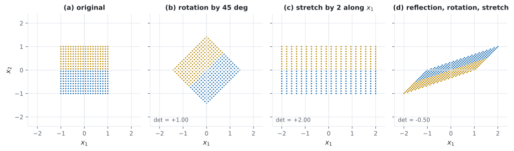
See it move

A rank-1 map squashes the whole plane onto a line. The amber line is the image; the red dashed line is the kernel — every point on it lands on the origin.

sketch Image and kernel of a linear map p5.js Pause Restart

The map Phi(x)=Ax with a rank-1 matrix squashes the entire input plane (blue lattice) onto one line, the image (amber). The red dashed line is the kernel: every point on it maps to the origin. dim(kernel) + dim(image) = 2.

Watch the probe. When the blue input crosses the red dashed line the amber output passes through the origin — that is what “the kernel maps to zero” looks like in motion. And no matter where the input goes, the output never leaves the amber line: the image is all the map can reach, and it is one-dimensional because the rank is 1.

Basis change, made concrete

The book’s Example 2.23 in the lab: a matrix that looks like a shear in the standard basis and is a pure diagonal scaling in the right one.

matrixThe matrix whose eigenbasis makes it diagonallinear map on R^2

2112

columns of A = images of e1, e2

det A 3area factor 3orientation preserved

1e1, e2 = (1, 0), (0, 1)          # the basis we start from2A @ e1  ==  A[:, 0]              # first column IS the image of e13A @ e2  ==  A[:, 1]              # second column IS the image of e24# linearity: A(x1 e1 + x2 e2) = x1 (A e1) + x2 (A e2)5det(A) = a*d - b*c               # signed area of the image of the unit square6A @ v = lam * v                  # an eigenvector keeps its direction

det A3A e1(2, 1)A e2(1, 2)

basisThe plane before anything happens, with the standard basis e1 = (1, 0) and e2 = (0, 1) and the unit square they span.

Play‹›1/8⟲

Its eigenvectors are (1,1) and (1,-1) with eigenvalues 3 and 1 — so in that basis it is diag(3, 1). Watch the eigen-directions in the final frame.

The last frame draws the eigen-directions, and they are exactly $(1,1)$ and $(1,-1)$ with eigenvalues $3$ and $1$. Those numbers are the diagonal of $\tilde{\mathbf{A}}$. Basis change and eigendecomposition are the same operation seen from two sides — §4.4 makes it official.

From scratch

linear_mappings.py

import numpy as np
 
rng = np.random.default_rng(0)
 
def is_linear(phi, dim, trials=500, tol=1e-9):
    """Test the single linearity condition on random inputs and scalars."""
    for _ in range(trials):
        x, y = rng.standard_normal(dim), rng.standard_normal(dim)
        lam, psi = rng.normal(), rng.normal()
        lhs = phi(lam * x + psi * y)
        rhs = lam * np.asarray(phi(x)) + psi * np.asarray(phi(y))
        if not np.allclose(lhs, rhs, atol=tol):
            return False
    return True
 
# ---- the zero test disqualifies fastest ------------------------------
cands = {
    "3x            ": lambda v: 3 * v,
    "3x + 1        ": lambda v: 3 * v + 1,
    "x squared     ": lambda v: v ** 2,
    "cos(x)        ": lambda v: np.cos(v),
    "A @ x         ": lambda v: np.array([[1.0, 2.0], [3.0, 4.0]]) @ v,
}
for name, f in cands.items():
    z = np.asarray(f(np.zeros(2)))
    sends_zero = np.allclose(z, 0)
    print(f"{name} Phi(0)=0: {str(sends_zero):5s}  linear: {is_linear(f, 2)}")
 
# ---- coordinates with respect to an ordered basis --------------------
x = np.array([2.0, 3.0])
B = np.array([[1.0, 1.0], [-1.0, 1.0]])        # columns b1=(1,-1), b2=(1,1)
alpha = np.linalg.solve(B, x)
print("\ncoordinates of (2,3) in B:", alpha, " = 0.5 * ", 2 * alpha)
print("rebuild:", B @ alpha, " matches x:", np.allclose(B @ alpha, x))
 
# Ordering matters: swap the basis vectors and the coordinate list swaps.
B_swapped = B[:, ::-1]
print("with the basis vectors swapped:", np.linalg.solve(B_swapped, x))
 
# ---- the transformation matrix's columns ----------------------------
A = np.array([[1.0, 2.0], [3.0, 4.0]])
for j, e in enumerate(np.eye(2)):
    print(f"\nPhi(e{j+1}) =", A @ e, " == column {}: {}".format(j, A[:, j]))
 
# ---- basis change: the book's Example 2.23 -------------------------
A23 = np.array([[2.0, 1.0], [1.0, 2.0]])
S = np.array([[1.0, 1.0], [1.0, -1.0]])        # new basis vectors as columns
A_tilde = np.linalg.inv(S) @ A23 @ S
print("\nExample 2.23:")
print("A in the canonical basis:\n", A23)
print("A in the basis ((1,1),(1,-1)):\n", np.round(A_tilde, 12))
print("diagonal?", np.allclose(A_tilde, np.diag(np.diag(A_tilde))))
vals, vecs = np.linalg.eigh(A23)
print("eigenvalues:", vals, " -> the diagonal entries, in the other order")
 
# ---- the book's Example 2.24, all the way through ------------------
A24 = np.array([[1.0, 2.0, 0.0],
                [-1.0, 1.0, 3.0],
                [3.0, 7.0, 1.0],
                [-1.0, 2.0, 4.0]])
S24 = np.array([[1.0, 0.0, 1.0],
                [1.0, 1.0, 0.0],
                [0.0, 1.0, 1.0]])
T24 = np.array([[1.0, 1.0, 0.0, 1.0],
                [1.0, 0.0, 1.0, 0.0],
                [0.0, 1.0, 1.0, 0.0],
                [0.0, 0.0, 0.0, 1.0]])
A24_tilde = np.linalg.inv(T24) @ A24 @ S24
print("\nExample 2.24, T^-1 A S =\n", np.round(A24_tilde, 10))
 
# ---- image, kernel, rank-nullity: the book's Example 2.25 ---------
A25 = np.array([[1.0, 2.0, -1.0, 0.0],
                [1.0, 0.0,  0.0, 1.0]])
r = np.linalg.matrix_rank(A25)
n = A25.shape[1]
k1 = np.array([0.0, 0.5, 1.0, 0.0])
k2 = np.array([-1.0, 0.5, 0.0, 1.0])
print("\nExample 2.25:")
print("rank = dim(Im) :", r, " (all of R^2)")
print("dim(ker)       :", n - r)
print("k1 in kernel   :", np.allclose(A25 @ k1, 0), " k2 in kernel:", np.allclose(A25 @ k2, 0))
print("rank-nullity   :", (n - r), "+", r, "=", n, " == dim(V):", n)
 
# ---- injective iff surjective iff bijective, for SQUARE only ------
print("\nsquare, full rank      -> all three:", end=" ")
Sq = np.array([[1.0, 2.0], [3.0, 4.0]])
rk = np.linalg.matrix_rank(Sq)
print(f"rank {rk} of 2, injective={rk==2}, surjective={rk==2}")
print("non-square, tall       -> can be injective and NOT surjective:", end=" ")
Tall = np.array([[1.0], [2.0], [3.0]])
print(f"rank {np.linalg.matrix_rank(Tall)}, image is a line in R^3")
print("non-square, wide       -> surjective and NOT injective:", end=" ")
print(f"rank {r} of R^2 reached, but kernel has dim {n - r}")

text

3x             Phi(0)=0: True   linear: True
3x + 1         Phi(0)=0: False  linear: False
x squared      Phi(0)=0: True   linear: False
cos(x)         Phi(0)=0: False  linear: False
A @ x          Phi(0)=0: True   linear: True
 
coordinates of (2,3) in B: [-0.5  2.5]  = 0.5 *  [-1.  5.]
rebuild: [2. 3.]  matches x: True
with the basis vectors swapped: [ 2.5 -0.5]
 
Phi(e1) = [1. 3.]  == column 0: [1. 3.]
 
Phi(e2) = [2. 4.]  == column 1: [2. 4.]
 
Example 2.23:
A in the canonical basis:
 [[2. 1.]
 [1. 2.]]
A in the basis ((1,1),(1,-1)):
 [[3. 0.]
 [0. 1.]]
diagonal? True
eigenvalues: [1. 3.]  -> the diagonal entries, in the other order
 
Example 2.24, T^-1 A S =
 [[-4. -4. -2.]
 [ 6.  0.  0.]
 [ 4.  8.  4.]
 [ 1.  6.  3.]]
 
Example 2.25:
rank = dim(Im) : 2  (all of R^2)
dim(ker)       : 2
k1 in kernel   : True  k2 in kernel: True
rank-nullity   : 2 + 2 = 4  == dim(V): 4
 
square, full rank      -> all three: rank 2 of 2, injective=True, surjective=True
non-square, tall       -> can be injective and NOT surjective: rank 1, image is a line in R^3
non-square, wide       -> surjective and NOT injective: rank 2 of R^2 reached, but kernel has dim 2

Four things confirmed against the book.

The zero test does real work. 3x + 1 and cos(x) are eliminated by one evaluation each, and x squared survives the zero test and fails linearity — so the test is necessary but not sufficient, exactly as expected.

Coordinates depend on the ordering. $(-0.5, 2.5) = \tfrac12(-1, 5)$ reproduces Example 2.20, and swapping the two basis vectors swaps the coordinate list to $(2.5, -0.5)$. Same point, same basis set, different basis tuple, different answer.

Example 2.23 comes out diagonal, $\operatorname{diag}(3, 1)$, and the eigenvalues are $1$ and $3$ — the same numbers, in the order eigh chose to return them. Basis change found the eigenbasis without being asked.

Example 2.24 reproduces the book’s $\tilde{\mathbf{A}}_\Phi$ exactly, including the awkward $(-4, -4, -2)$ first row.

On real data

figure The book's Figure 2.10, reproduced matplotlib

Four hundred points, three matrices. Straight lines stay straight and evenly spaced lines stay evenly spaced in every panel — that is what linearity looks like.

figure Rank-nullity as a conservation law matplotlib

For every matrix the two bars sum to the number of columns. Every input dimension either survives into the image or is crushed into the kernel.

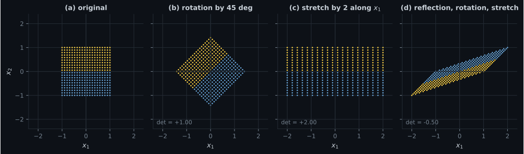
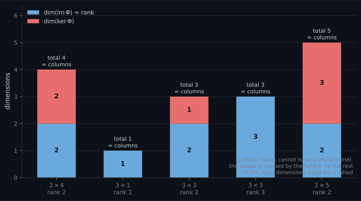
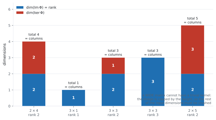
Reading the plot

The second figure is rank-nullity drawn as a conservation law, which is the most useful way to hold it. Each bar’s total height is $\dim(V)$ — the number of columns — and the split between image and kernel varies with the rank. The total never does.

That framing makes the consequences immediate rather than something to derive. A wide matrix ($n > m$) cannot have a trivial kernel, because the image dimension is capped at $m < n$ and the rest of $n$ has to go somewhere. So a wide matrix is never injective — there are always distinct inputs colliding on the same output. That is precisely why an under-determined system has infinitely many solutions (§2.1), and why a compression step is inherently lossy (Chapter 10).

Conversely a tall matrix ($m > n$) can have a trivial kernel and still fail to be surjective, because the image is at most $n$-dimensional inside an $m$-dimensional codomain. That is why an overdetermined system usually has no solution.

The three-way equivalence — injective iff surjective iff bijective — needs $\dim(V) = \dim(W)$, and the figure shows why: only when the bar height equals the codomain dimension can filling one force the other.

From the book

Mathematics for Machine Learning §2.7 opens with the structure-preservation conditions (Equations 2.85–2.86) and Definition 2.15 (linear mapping / vector space homomorphism / linear transformation, Equation 2.87). Definition 2.16 gives injective, surjective and bijective, followed by the special cases isomorphism, endomorphism, automorphism and the identity mapping $\mathrm{id}_V$. Example 2.19 shows $\Phi(\mathbf{x}) = x_1 + ix_2$ is a homomorphism (Equation 2.88) and remarks that this “justifies why complex numbers can be represented as tuples in $\mathbb{R}^2$”. Theorem 2.17 states that finite-dimensional $V$ and $W$ are isomorphic iff $\dim(V) = \dim(W)$, with the remark that such spaces “are kind of the same thing” and the justification for treating $\mathbb{R}^{m\times n}$ and $\mathbb{R}^{mn}$ alike; further remarks note that compositions of linear mappings are linear, the inverse of an isomorphism is an isomorphism, and $\Phi+\Psi$ and $\lambda\Phi$ are linear. §2.7.1 introduces the ordered basis (Equation 2.89) with the notation remark distinguishing $B$ (tuple), $\mathcal{B}$ (set) and $\mathbf{B}$ (matrix), then Definition 2.18 (coordinates, Equations 2.90–2.91) and Figure 2.8; Example 2.20 with Figure 2.9 gives $\mathbf{x} = (2,3)^\top$ having coordinates $\tfrac12(-1,5)^\top$ in the basis $\bigl((1,-1)^\top,(1,1)^\top\bigr)$. Definition 2.19 is the transformation matrix (Equations 2.92–2.93) with $\hat{\mathbf{y}} = \mathbf{A}_\Phi\hat{\mathbf{x}}$ (Equation 2.94); Example 2.21 computes one (Equations 2.95–2.96) and Example 2.22 with Figure 2.10 applies three transformation matrices to 400 vectors arranged in a square (Equation 2.97). §2.7.2 gives Example 2.23, where $\begin{bmatrix}2&1\\1&2\end{bmatrix}$ becomes $\begin{bmatrix}3&0\\0&1\end{bmatrix}$ in the basis $\bigl((1,1)^\top,(1,-1)^\top\bigr)$ (Equations 2.100–2.102), and Theorem 2.20 (Basis Change, Equation 2.105) $\tilde{\mathbf{A}}_\Phi = \mathbf{T}^{-1}\mathbf{A}_\Phi\mathbf{S}$ with its proof (Equations 2.106–2.113) and Figure 2.11; Definition 2.21 (equivalence) and Definition 2.22 (similarity) follow, with the remark that similar matrices are always equivalent but not conversely, and that $\mathbf{A}_{\Psi\circ\Phi} = \mathbf{A}_\Psi\mathbf{A}_\Phi$. Example 2.24 works a full basis change (Equations 2.117–2.121b). §2.7.3 gives Definition 2.23 (image and kernel, Equations 2.122–2.123) with Figure 2.12, the remarks that $\mathbf{0}_V \in \ker(\Phi)$ so the null space is never empty, that both are subspaces, and that $\Phi$ is injective iff $\ker(\Phi) = \{\mathbf{0}\}$; the Null Space and Column Space remark identifies $\operatorname{Im}(\Phi)$ with the column space (Equations 2.124a–b) and notes $\operatorname{rk}(\mathbf{A}) = \dim(\operatorname{Im}(\Phi))$, that the kernel is the general solution of $\mathbf{A}\mathbf{x} = \mathbf{0}$, and that the kernel is a subspace of $\mathbb{R}^n$ where $n$ is the “width” of the matrix. Example 2.25 computes both for a $2\times4$ matrix (Equations 2.125a–2.128). Theorem 2.24 is the rank-nullity theorem (Equation 2.129), also called the fundamental theorem of linear mappings, with the three consequences listed above.

Pitfalls

A mapping with a constant offset is not linear

$\Phi(x) = 3x + 1$ fails, because $\Phi(0) = 1 \neq 0$. It is affine (§2.8). This matters constantly in practice: a neural network layer $\mathbf{W}\mathbf{x} + \mathbf{b}$ is affine, not linear, and the bias is exactly the offset. Papers still call these “linear layers”.

The transformation matrix depends on both bases

“The matrix of $\Phi$” is incomplete phrasing. There is a matrix per pair of ordered bases, related by $\tilde{\mathbf{A}} = \mathbf{T}^{-1}\mathbf{A}\mathbf{S}$. When both bases are standard the distinction is invisible, which is why it causes so much trouble when it stops being.

Matrix multiplication maps coordinates, not vectors

$\hat{\mathbf{y}} = \mathbf{A}_\Phi\hat{\mathbf{x}}$ relates coordinate vectors. The underlying vectors live in $V$ and $W$ and never touch a matrix. Conflating the two is the root of most basis-change confusion.

Kernel and image live in different spaces

The kernel is a subspace of $\mathbb{R}^n$ — the width. The image is a subspace of $\mathbb{R}^m$ — the height. Getting this backwards makes rank-nullity look dimensionally inconsistent. And note the kernel is never empty: it always contains $\mathbf{0}$.

Injective iff surjective needs equal dimensions

The three-way equivalence holds only when $\dim(V) = \dim(W)$. A wide matrix is never injective and a tall one is rarely surjective, and both statements follow from rank-nullity plus the cap $\dim(\operatorname{Im}) \le \min(m,n)$.

Compare

shape	typical rank	kernel	injective?	surjective?
square, full rank	$n$	$\{\mathbf{0}\}$	yes	yes — and bijective
square, deficient	$< n$	non-trivial	no	no
tall, $m > n$, full rank	$n$	$\{\mathbf{0}\}$	yes	no — image is $n$-dim in $\mathbb{R}^m$
wide, $n > m$, full rank	$m$	dimension $n - m \ge 1$	no	yes

The two middle-column entries in the last two rows are the asymmetry the figure makes visible: a tall matrix loses nothing and reaches little; a wide one reaches everything and loses information.

pch.quizTag Check yourself

1. What is the fastest way to show a mapping is not linear?

   A Check additivity on two random vectors B Check whether it sends the zero vector to the zero vector C Compute its rank D Check whether it is injective
   pch.quizShowAnswer

   B — Check whether it sends the zero vector to the zero vector — Linearity forces Phi(0) = 0, so any mapping with a constant offset is disqualified by one evaluation. It is necessary but not sufficient — x squared passes the zero test and is still not linear.

2. What does the j-th column of a transformation matrix contain?

   A The j-th basis vector of the domain B The coordinates of the image of the j-th domain basis vector, with respect to the codomain basis C The j-th eigenvector D The j-th row of the inverse
   pch.quizShowAnswer

   B — The coordinates of the image of the j-th domain basis vector, with respect to the codomain basis — That is the definition. It is section 2.2's 'columns are the images of the basis vectors', made precise — with the important caveat that 'images' means in coordinates, and which coordinates depends on the codomain basis.

3. A four-by-six matrix has full rank. What can you say?

   A It is injective but not surjective B It is surjective but not injective — the kernel has dimension two C It is bijective D Neither, without more information
   pch.quizShowAnswer

   B — It is surjective but not injective — the kernel has dimension two — Four rows and six columns means the image is at most four-dimensional and full rank makes it exactly four, so it covers the codomain. Rank-nullity then forces the kernel to have dimension six minus four, so distinct inputs collide.

4. Why does anyone bother changing basis?

   A To make the matrix smaller B Because the same mapping can have a far simpler matrix in the right basis — the book's example turns a shear-looking matrix into a diagonal one C Because the standard basis is not a real basis D To make the mapping injective
   pch.quizShowAnswer

   B — Because the same mapping can have a far simpler matrix in the right basis — the book's example turns a shear-looking matrix into a diagonal one — The mapping does not change; the description does. A diagonal matrix raised to a high power is trivial, which is the entire motivation for Chapter 4's diagonalisation and for Chapter 10's choice of a basis in which data compresses.

🧪 Try It Yourself

Exercise 1 – The zero test

pch.exerciseTag pch.exerciseTitle

Exercise 2 – Coordinates depend on the ordering

pch.exerciseTag pch.exerciseTitle

Exercise 3 – Basis change can diagonalise

pch.exerciseTag pch.exerciseTitle

Exercise 4 – Rank-nullity as a conservation law

pch.exerciseTag pch.exerciseTitle

Exercise 5 – Verify a kernel basis

pch.exerciseTag pch.exerciseTitle

Recall card

• Linearity is one condition — the mapping commutes with taking linear combinations — and it packages additivity and homogeneity together.
• Every linear mapping sends zero to zero, which is the cheapest disqualifier: any constant offset makes a mapping affine rather than linear.
• Isomorphism is linear plus bijective; endomorphism maps a space to itself; automorphism is both.
• Two finite-dimensional spaces are isomorphic exactly when their dimensions agree, which is why an m-by-n matrix space can be treated as a vector space of length mn.
• A basis must be ordered because coordinates are a list — swapping two basis vectors swaps the coordinates of every point.
• The j-th column of the transformation matrix is the coordinates of the image of the j-th basis vector, expressed in the codomain basis.
• Matrix multiplication maps coordinates, not vectors — the underlying vectors never touch a matrix.
• Basis change is T inverse times A times S, read right to left: translate in, map, translate out.
• Similar means the same matrix on both sides; equivalent allows different ones. Similar implies equivalent, not conversely.
• The kernel lives in the width and the image in the height — different spaces, which is why rank-nullity needs care.
• The kernel is never empty; it always contains the zero vector, and the mapping is injective exactly when that is all it contains.
• Rank-nullity is a conservation law: image dimension plus kernel dimension equals the number of input dimensions, always.
• A wide matrix is never injective and a tall one is rarely surjective, and injective-iff-surjective-iff-bijective needs the two dimensions to match.

Next: what happens when the offset is allowed back in — Affine Spaces.