Decision Trees - Entropy and Gini Impurity

What you’ll learn

• how a tree turns a dataset into a list of if-statements you can read aloud
• Gini impurity and entropy — the formulas, and the real difference between them
• both computed by hand on the actual iris tree, matching scikit-learn to six decimals
• how CART searches for a split, and why the result is only locally optimal
• why an unpruned tree always reaches 100% training accuracy, and every control that prevents it
• why trees are unstable, and what that instability sets up for Phase 5

Intuition

A decision tree asks a sequence of yes/no questions about one feature at a time, and each answer narrows the possibilities until only one class remains plausible. It is the only model in this phase whose reasoning you can print and hand to a domain expert:

text

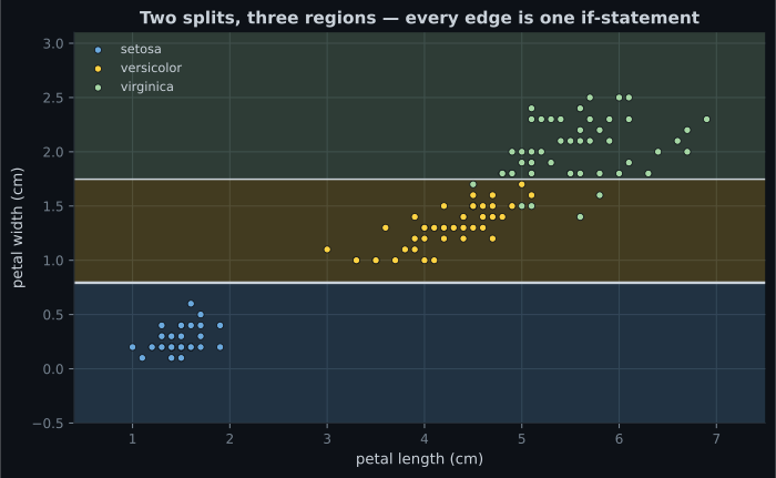
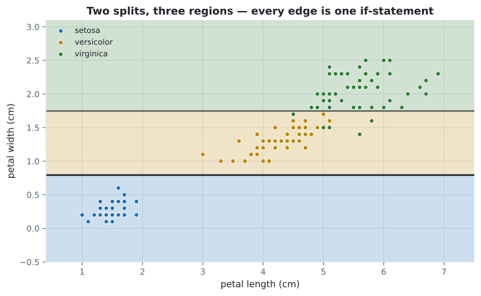
if petal width <= 0.80:
    setosa
else:
    if petal width <= 1.75:
        versicolor
    else:
        virginica

Two questions, three answers, 96% accurate on the full iris dataset. No scaling, no distance metric, no kernel, no probability calibration — just thresholds.

The whole design problem is: which question, in which order? That is what impurity measures answer.

diagram Diagram mermaid

  flowchart TD
  A["150 samples
50 / 50 / 50
gini 0.667"] -->|"petal width ≤ 0.8"| B["50 samples
all setosa
gini 0.000"]
  A -->|"petal width > 0.8"| C["100 samples
0 / 50 / 50
gini 0.500"]
  C -->|"petal width ≤ 1.75"| D["54 samples
0 / 49 / 5
gini 0.168"]
  C -->|"petal width > 1.75"| E["46 samples
0 / 1 / 45
gini 0.043"]

The math

Measuring impurity

A node is pure if every sample in it shares a label. Impurity measures how far from that a node is. With $p_c$ the proportion of class $c$ in the node:

$$G = 1 - \sum_{c=1}^{K} p_c^2 \qquad\qquad H = -\sum_{c=1}^{K} p_c \log_2 p_c$$

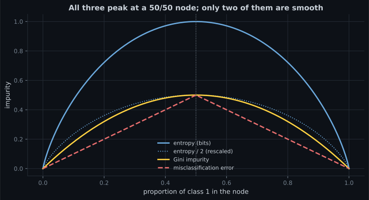
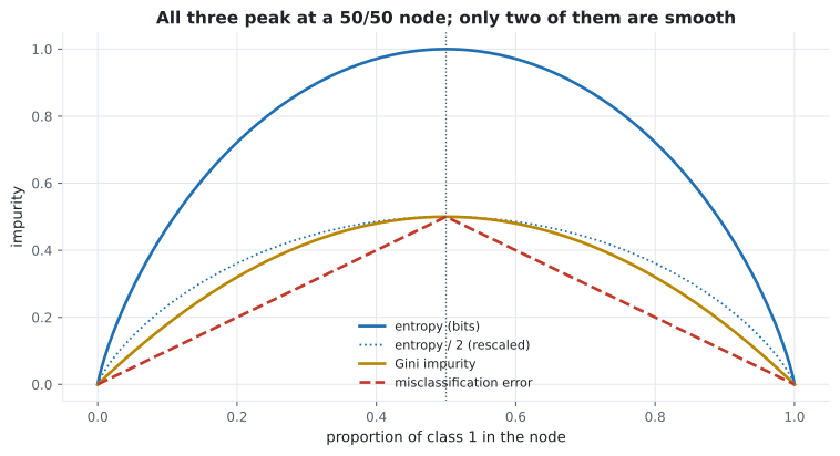
Both are zero for a pure node and maximal for a uniform one. Their maxima differ: for $K$ classes, Gini tops out at $1 - 1/K$ while entropy tops out at $\log_2 K$. With three classes that is 0.667 against 1.585.

figure Three impurity measures over a binary node matplotlib

Rescale entropy by half and it nearly overlays Gini — which is why the choice rarely changes the tree. Misclassification error has a corner at 0.5 and a flat gradient, so it is a poor splitting criterion.

Reading the plot

• Gini and entropy agree almost everywhere. After rescaling, the two curves are close enough that they select the same split the overwhelming majority of the time. Gini is marginally faster because it avoids a logarithm; that is the entire practical difference.
• Entropy is slightly more aggressive at the extremes, so it can prefer a split that isolates a small pure group where Gini would not.
• Misclassification error is flat over wide ranges. Two candidate splits often score identically, so it gives the search nothing to descend. It is used for pruning, not for growing.

Choosing a split

CART evaluates every (feature, threshold) pair and picks the one minimising the weighted impurity of the two children:

$$J(k, t_k) = \frac{m_{\text{left}}}{m}\,G_{\text{left}} + \frac{m_{\text{right}}}{m}\,G_{\text{right}}$$

The information gain is the parent’s impurity minus that weighted average. Split, then recurse on each child, stopping when a node is pure or a limit is reached.

Two properties follow directly:

• It is greedy. Each split is chosen to be locally best; nothing looks two moves ahead. Finding the globally optimal tree is NP-complete, so every practical tree is a good local solution.
• It is invariant to monotone transformations. Only the ordering of a feature’s values matters, never the spacing. Log-transform a feature, or standardise it, and the tree is unchanged. This is why trees never need scaling.

Worked example by hand

The iris tree above, computed from scratch.

Step 1 — root impurity. 150 samples, 50 of each class:

$$G_{\text{root}} = 1 - \left(\tfrac{50}{150}\right)^2 - \left(\tfrac{50}{150}\right)^2 - \left(\tfrac{50}{150}\right)^2 = 1 - 3\left(\tfrac{1}{9}\right) = \tfrac{2}{3} \approx 0.6667$$

Step 2 — evaluate the split at petal width ≤ 0.80. The left child gets 50 setosa and nothing else; the right child gets 50 versicolor and 50 virginica:

$$G_{\text{left}} = 1 - 1^2 = 0, \qquad G_{\text{right}} = 1 - 0.5^2 - 0.5^2 = 0.5$$ $$J = \frac{50}{150}(0) + \frac{100}{150}(0.5) = 0.3333$$ $$\text{gain} = 0.6667 - 0.3333 = 0.3333$$

No other threshold on either feature beats that, so CART takes it.

Step 3 — split the right child at petal width ≤ 1.75. The 100 remaining samples divide into 54 (49 versicolor, 5 virginica) and 46 (1 versicolor, 45 virginica):

$$G_{\text{left}} = 1 - \left(\tfrac{49}{54}\right)^2 - \left(\tfrac{5}{54}\right)^2 = 1 - 0.8234 - 0.0086 = 0.1680$$ $$G_{\text{right}} = 1 - \left(\tfrac{1}{46}\right)^2 - \left(\tfrac{45}{46}\right)^2 = 1 - 0.0005 - 0.9570 = 0.0425$$ $$J = \frac{54}{100}(0.1680) + \frac{46}{100}(0.0425) = 0.0907 + 0.0196 = 0.1103$$ $$\text{gain} = 0.5 - 0.1103 = 0.3897$$

Every one of these numbers is available from the fitted estimator as tree_.impurity, and they agree to six decimal places.

The same tree by entropy. $H_{\text{root}} = \log_2 3 = 1.5850$, the right child is $H = 1.0000$, and the two leaves are 0.4451 and 0.1511. Different scale, identical thresholds: 0.80 and 1.75.

figure The same tree, drawn in feature space matplotlib

Two splits, three rectangles. Both cuts are horizontal because both use petal width — the tree found petal length unnecessary.

See it move

sketch Splitting a node to reduce impurity p5.js Pause Restart

A node of mixed points is split by a threshold; the bars show the impurity of each child and the weighted average the split achieves. The best threshold is the one that minimises the bar on the right.

From scratch

tree_splits.py

import numpy as np
 
 
def gini(labels):
    if len(labels) == 0:
        return 0.0
    _, counts = np.unique(labels, return_counts=True)
    p = counts / counts.sum()
    return float(1 - (p**2).sum())
 
 
def entropy(labels):
    if len(labels) == 0:
        return 0.0
    _, counts = np.unique(labels, return_counts=True)
    p = counts / counts.sum()
    return float(-(p * np.log2(p)).sum())
 
 
def best_split(X, y, impurity=gini):
    """Exhaustive search over every feature and every midpoint threshold."""
    best = (None, None, impurity(y))
    m = len(y)
    for feature in range(X.shape[1]):
        values = np.unique(X[:, feature])
        thresholds = (values[:-1] + values[1:]) / 2      # midpoints
        for t in thresholds:
            mask = X[:, feature] <= t
            if mask.sum() == 0 or (~mask).sum() == 0:
                continue
            weighted = (mask.sum() * impurity(y[mask])
                        + (~mask).sum() * impurity(y[~mask])) / m
            if weighted < best[2]:
                best = (feature, float(t), weighted)
    return best
 
 
from sklearn.datasets import load_iris
 
iris = load_iris()
X = iris.data[:, (2, 3)]          # petal length, petal width
y = iris.target
 
print(f"root gini = {gini(y):.6f}")                  # root gini = 0.666667
feature, threshold, weighted = best_split(X, y)
print(f"split on feature {feature} at {threshold:.2f}")   # feature 1 at 0.80
print(f"weighted impurity = {weighted:.6f}")              # 0.333333
print(f"information gain  = {gini(y) - weighted:.6f}")    # 0.333333

Forty lines reproduce scikit-learn’s first split exactly, threshold included.

Trees overfit, aggressively

figure max_depth = 1, 4 and unlimited matplotlib

An unlimited tree keeps splitting until every leaf is pure, which on noisy data means one leaf per noisy point. Training accuracy 1.00, and a boundary nobody would trust.

figure Where learning stops and memorising starts matplotlib

Training accuracy reaches 1.0 and never moves again. Cross-validated accuracy peaks at a shallow depth and then falls — every split past that point is fitting noise.

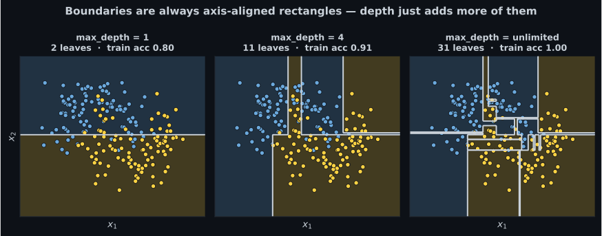
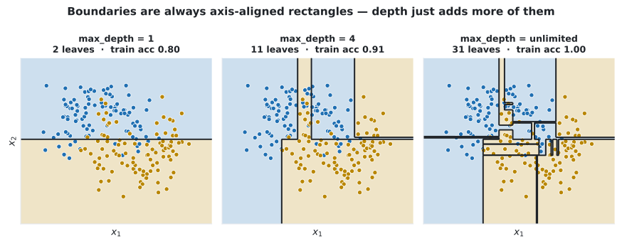
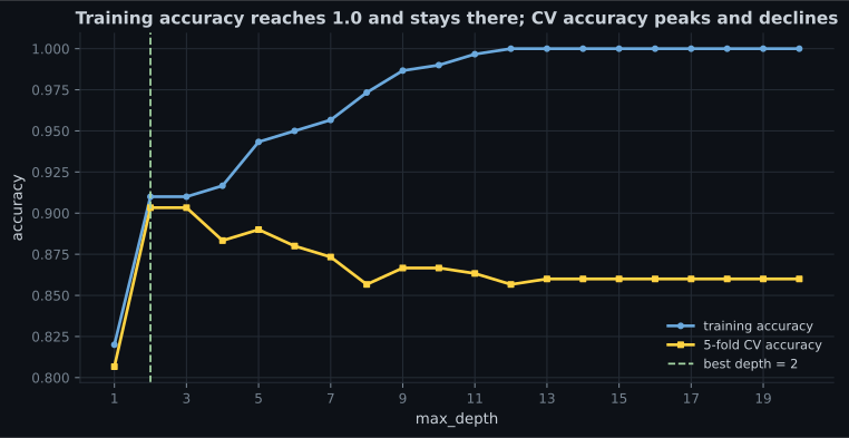
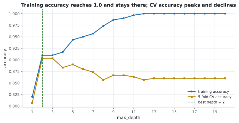
An unpruned tree will always reach 100% training accuracy on data with no duplicated rows, because it can keep splitting until each leaf holds one sample. That is not a bug in the implementation; it is what “grow until pure” means. The controls that prevent it:

Parameter	Effect	Typical value
max_depth	Hard cap on tree height	3–10
min_samples_split	Refuse to split a node below this size	10–50
min_samples_leaf	Every leaf must hold at least this many	5–20
max_leaf_nodes	Cap total leaves; grows best-first instead of depth-first	10–50
min_impurity_decrease	Refuse a split that gains less than this	0.0–0.01
ccp_alpha	Cost-complexity pruning after growing	Tune via cost_complexity_pruning_path

min_samples_leaf is the most reliable single knob: it directly forbids the “one leaf per noisy point” failure, whatever the depth.

pruning.py

from sklearn.datasets import load_iris
from sklearn.model_selection import cross_val_score
from sklearn.tree import DecisionTreeClassifier
 
iris = load_iris()
X, y = iris.data[:, (2, 3)], iris.target
 
for depth in (1, 2, 3, 5, None):
    model = DecisionTreeClassifier(max_depth=depth, random_state=0)
    train = model.fit(X, y).score(X, y)
    cv = cross_val_score(model, X, y, cv=5).mean()
    print(f"depth={str(depth):<5} leaves {model.get_n_leaves():2d}"
          f"  train {train:.4f}  cv {cv:.4f}")
 
# depth=1     leaves  2  train 0.6667  cv 0.6667
# depth=2     leaves  3  train 0.9600  cv 0.9600
# depth=3     leaves  5  train 0.9733  cv 0.9600
# depth=5     leaves  8  train 0.9933  cv 0.9533
# depth=None  leaves  8  train 0.9933  cv 0.9467

Depth 2 already achieves the best cross-validated score. Everything past it buys training accuracy and loses generalisation — three extra splits to gain 0.033 on training data and lose 0.013 on held-out data.

Instability

Trees are high variance: resample the training data slightly and you can get a completely different tree. The cause is the greedy search — if two candidate splits score almost equally at the root, a handful of different rows flips which one wins, and every subsequent split changes.

This is a genuine weakness, and it is also the opening for Phase 5. If a model’s errors change substantially with the training sample, averaging many of them cancels the variance out. That single observation is what a random forest is.

pch.algoTag Decision Tree (CART) Supervised · Classification and Regression

pch.algoApi sklearn.tree.DecisionTreeClassifier

pch.algoAssumes

• The target can be approximated by axis-aligned rectangular regions
• Feature ordering is meaningful; spacing need not be
• Enough samples per leaf for the leaf proportions to mean something

pch.algoCost

pch.algoTrain

O(n · m log m)

pch.algoPredict

O(depth)

pch.algoMemory

O(nodes)

m = samples, n = features; prediction is logarithmic in a balanced tree

pch.algoHyperparams

• max_depth default None None means grow until pure, which guarantees overfitting. Set it.
• min_samples_leaf default 1 The most effective single guard against memorising individual points. Try 5 to 20.
• criterion default gini 'entropy' is marginally more aggressive at the extremes and slightly slower. Rarely changes the result.
• ccp_alpha default 0.0 Cost-complexity pruning after growing. Use cost_complexity_pruning_path to get candidate values.
• class_weight default None 'balanced' reweights impurity by inverse class frequency on imbalanced data.

pch.algoReachFor

• You need a model a non-technical stakeholder can read
• Features are a mix of scales and types and you do not want to preprocess
• You want a base learner for a forest or a boosted ensemble
• Non-linear interactions matter and you want them found automatically

pch.algoLookElsewhere

• You need a smooth or diagonal boundary — a tree approximates one with a staircase
• The dataset is small and stability matters
• You need to extrapolate beyond the training range; a tree predicts a constant outside it
• A single model's accuracy is the priority — use an ensemble

Pitfalls

Leaving max_depth=None

The default grows until every leaf is pure. On any real dataset that is guaranteed overfitting, and the training score will look wonderful. Always set max_depth or min_samples_leaf.

feature_importances_ is biased

Impurity-based importance favours high-cardinality features — a continuous feature offers hundreds of candidate thresholds while a binary one offers exactly one, so the continuous feature wins splits by having more chances. Prefer permutation importance when the ranking actually matters.

Trees cannot extrapolate

A leaf predicts a constant. Beyond the training range that constant never changes, so a regression tree fitted on prices from 100k to 500k will predict 500k for a mansion worth ten million. Linear models extrapolate wrongly; trees do not extrapolate at all.

A different random seed can give a different tree

When several splits tie, random_state breaks the tie. Two “identical” trees can have different structures. Set the seed, and do not read deep meaning into which of two near-equal features was chosen.

Compare

Model	Needs scaling	Handles categoricals	Interpretable	Boundary	Stability
Decision Tree	No	Natively, once encoded	Very, when shallow	Axis-aligned steps	Low
Random Forest	No	Yes	Poor	Many steps averaged	High
Logistic Regression	Yes	Needs one-hot	High	Linear	High
SVM (RBF)	Critically	Needs one-hot	Low	Smooth	Moderate
KNN	Critically	Needs encoding	Low	Local	Moderate

pch.quizTag pch.quizDefaultTitle

1. Why do decision trees not require feature scaling?

   A Because scikit-learn scales internally B Because a split depends only on the ordering of a feature's values, not on their spacing C Because impurity measures normalise the features D They do require scaling; omitting it is a common mistake
   pch.quizShowAnswer

   B — Because a split depends only on the ordering of a feature's values, not on their spacing — A threshold test asks whether x is above or below a value. Any monotone transformation — log, standardisation, squaring positives — preserves the ordering and therefore the tree.

2. A node contains 54 samples: 49 of class 1 and 5 of class 2. What is its Gini impurity?

   A 0.000 B 0.168 C 0.500 D 0.907
   pch.quizShowAnswer

   B — 0.168 — 1 - (49/54)² - (5/54)² = 1 - 0.8234 - 0.0086 = 0.1680. Mostly pure, so the impurity is low but not zero.

3. Why does an unpruned decision tree reach 100% training accuracy?

   A Because CART finds the globally optimal tree B Because it keeps splitting until every leaf is pure, which it can always do if no two rows are identical with different labels C Because Gini impurity is minimised globally D Because of a bug in the default parameters
   pch.quizShowAnswer

   B — Because it keeps splitting until every leaf is pure, which it can always do if no two rows are identical with different labels — 'Grow until pure' means exactly that. With enough splits every leaf can hold a single training point, so the training score is guaranteed and meaningless.

4. Two decision trees fitted on slightly different samples of the same data look completely different. What does that tell you, and what does it set up?

   A The data is corrupted B Trees are high variance because the greedy search amplifies small differences — which is exactly why averaging many of them works C The random seed was not set correctly D Trees should never be used
   pch.quizShowAnswer

   B — Trees are high variance because the greedy search amplifies small differences — which is exactly why averaging many of them works — A near-tie at the root flips under resampling and changes every subsequent split. High variance plus low bias is the ideal profile for bagging, which is what a random forest exploits.

🧪 Try It Yourself

Exercise 1 – Compute Gini impurity

pch.exerciseTag pch.exerciseTitle

Exercise 2 – Compute the information gain

pch.exerciseTag pch.exerciseTitle

Exercise 3 – Read the tree’s own numbers

pch.exerciseTag pch.exerciseTitle

Exercise 4 – Print the rules

pch.exerciseTag pch.exerciseTitle

Exercise 5 – Find where depth stops helping

pch.exerciseTag pch.exerciseTitle

Recap

• A tree is a sequence of single-feature threshold tests, readable as plain if-statements.
• Gini is $1 - \sum p_c^2$, entropy is $-\sum p_c \log_2 p_c$; after rescaling they nearly coincide, and they almost always choose the same split.
• Hand-worked on iris: root Gini 0.6667, first split gains 0.3333, second gains 0.3897 — matching tree_.impurity exactly.
• CART is greedy and only locally optimal; the globally best tree is NP-complete to find.
• Splits depend only on value ordering, so trees never need scaling.
• Unpruned trees always reach 100% training accuracy. On iris, depth 2 is the best cross-validated choice and depth 5 is already worse.
• Trees are unstable, and that instability is precisely what ensembles exploit.

Exercise 6 – Which hyperparameter actually matters?

pch.exerciseTag pch.exerciseTitle

Next

Continue to Naive Bayes Classifier — a probabilistic classifier that trains in one pass over the data and, despite an assumption that is essentially always false, remains hard to beat on text.