Intro to Recurrent Neural Networks (RNN) for Sequences

A dense layer sees a fixed-size vector with no notion of order. A convolution sees a fixed-size neighbourhood. A recurrent layer sees one element at a time and carries a state forward, so its output can depend on everything that came before.

That is the promise. This page measures the delivery, on 5,000 IMDB reviews truncated to 200 tokens, and the headline is uncomfortable: a SimpleRNN(32) scored 0.5856 while averaging the same embeddings and discarding order entirely scored 0.8004.

What you’ll learn

• The recurrence relation, and the same cell written in five lines of NumPy that match Keras to within 1e-6.
• What word order is worth, measured by destroying it: +0.0744 for the RNN, +0.0000 for a bag of words.
• What the hidden state actually does over 200 timesteps — including the fixed point it converges to while reading padding.
• Why return_sequences exists and when you need it.
• Where a SimpleRNN stops working, measured on the adding problem.
• Why the parameter count is independent of sequence length — and why the runtime is not.

The recurrence

$$h_t = \tanh\!\left(W_x x_t + W_h h_{t-1} + b\right), \qquad h_0 = \mathbf{0}$$

One weight matrix for the input, one for the previous state, one bias — shared across every timestep, which is what makes the layer independent of sequence length. The layer’s output is $h_T$, the state after the last element.

A SimpleRNN cell, from scratch

def simple_rnn(sequence, kernel, recurrent, bias):
    """sequence: (timesteps, features). Returns every hidden state."""
    h = np.zeros(kernel.shape[1], "float32")
    states = []
    for x in sequence:
        h = np.tanh(x @ kernel + h @ recurrent + bias)
        states.append(h.copy())
    return np.stack(states)

That loop is the layer. Exercise 2 runs it against keras.layers.SimpleRNN with the same weights and the two agree to 2.68e-07 — float32 rounding, nothing else. Worth confirming once, because everything else on this page follows from that single line.

The parameter count follows directly: for features inputs and units state,

$$\underbrace{\text{features} \times \text{units}}_{W_x} + \underbrace{\text{units}^2}_{W_h} + \underbrace{\text{units}}_{b}$$

so SimpleRNN(32) on 32-dimensional embeddings costs $32{\times}32 + 32^2 + 32 = 2{,}080$ parameters — regardless of whether the sequence is 20 steps or 20,000.

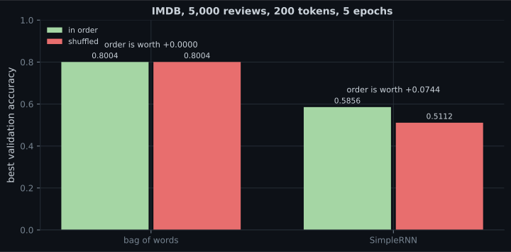
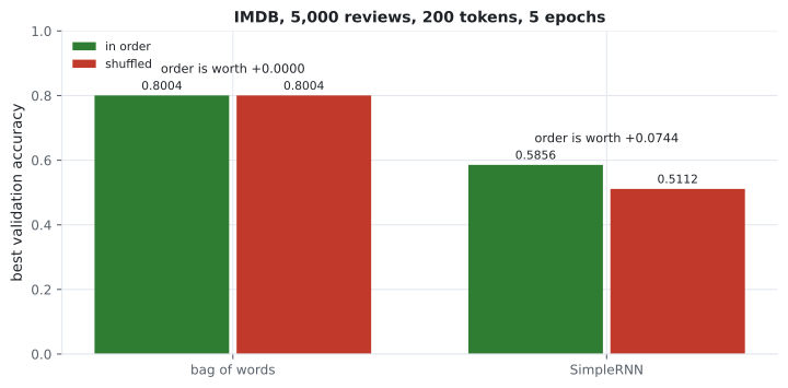
What is order actually worth?

The way to measure it is to destroy it. Shuffle the tokens inside every review — same words, same counts, no order — and retrain.

Model	In order	Shuffled	Order is worth
bag of words (GlobalAveragePooling1D)	0.8004	0.8004	+0.0000
SimpleRNN(32)	0.5856	0.5112	+0.0744

figure IMDB, 5,000 reviews, 200 tokens, 5 epochs matplotlib

Two results in one figure. The bag-of-words model is identical to four decimal places under shuffling — it must be, because averaging is permutation-invariant, and that identity is a useful check that the shuffle really happened. The SimpleRNN does use order, losing 0.0744 without it. And it is still 0.21 behind the model that has no idea what order is.

The honest reading:

1. Order carries real signal — the RNN’s 0.0744 drop proves it is using the sequence, not just the word counts.
2. A SimpleRNN is a bad way to extract that signal at 200 timesteps. Averaging the embeddings, which cannot represent “not good” differently from “good not”, beats it by 0.2148. The reason is the subject of the next page: a plain recurrent state cannot carry information across hundreds of steps.
3. The bag-of-words identity is the control. If the shuffled bag-of-words score had moved at all, the experiment would have been broken.

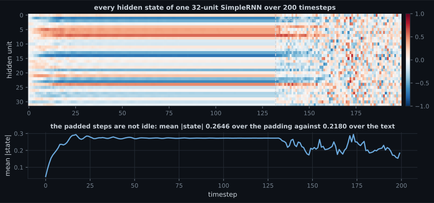
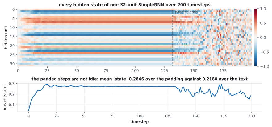
What the state does

Take one trained cell, rebuild it with return_sequences=True, copy the weights across and keep every $h_t$ for one review. This review is 68 tokens long inside a 200-step tensor, so it starts with 132 steps of padding.

figure Every hidden state of one 32-unit SimpleRNN over 200 timesteps matplotlib

The horizontal stripes are the important part: fed the same token 132 times, the recurrence converges to a fixed point and stops carrying information. Measured mean |state| is 0.2646 over the padding and 0.2180 over the actual review — the padded steps are not idle, they are saturated. Once real tokens arrive at step 132 the state becomes input-dependent again, which is exactly why pre-padding is survivable and post-padding is not.

Two measured facts worth keeping:

• The state is more active during padding than during text (0.2646 against 0.2180). Token id 0 has an ordinary embedding vector, and feeding it repeatedly drives the cell to $h^\* = \tanh(W_x x_{\text{pad}} + W_h h^\* + b)$ — an attractor.
• No unit saturated ($|h| > 0.99$) at the final step: 0 of 32. The tanh is being used in its linear-ish middle range here, which is not always true — a saturated unit has a near-zero gradient and stops learning.

That first point is the whole argument of the padding and masking page, and it is why the four setups there differ by 0.08 accuracy.

diagram Diagram mermaid

  flowchart LR
  X0["x₁"] --> C1["cell"]
  H0["h₀ = 0"] --> C1
  C1 --> H1["h₁"]
  X1["x₂"] --> C2["cell"]
  H1 --> C2
  C2 --> H2["h₂"]
  X2["x₃"] --> C3["cell"]
  H2 --> C3
  C3 --> H3["h₃ = output
(return_sequences=False)"]
  C1 -. "same Wx, Wh, b" .- C2
  C2 -. "same Wx, Wh, b" .- C3

return_sequences

Setting	Output shape	Use it for
False (default)	(batch, units) — the last state only	classification, one-step forecasting
True	(batch, timesteps, units) — every state	stacking recurrent layers, per-timestep labels, attention

Stacking is the common case, and it is a hard requirement: every recurrent layer except the last needs return_sequences=True, or the next layer receives a vector where it expects a sequence.

Where it stops working

Sentiment does not need long-range memory, so it cannot show where a SimpleRNN breaks. The adding problem can: a sequence of uniform values with two marked positions — one near the start, one in the second half — where the target is the sum of the two marked values. Carrying a number across the sequence is the task, and predicting the mean sum of 1.0 is the do-nothing baseline.

Sequence length	Baseline MAE	SimpleRNN(32)	LSTM(32)
10	0.3167	0.0241	0.0074
40	0.3255	0.0641	0.0109
100	0.3233	0.3106 ← at the baseline	0.0152
200	0.3287	0.3289	0.3173

figure The adding problem — 3,000 sequences, 60 epochs, 32 units matplotlib

The SimpleRNN solves the task at 10 and 40 steps, then collapses onto the baseline at 100: it has not merely got worse, it has stopped carrying the number at all. The LSTM holds to 100 steps at MAE 0.0152 — twenty times better — and then fails too at 200. That last column is honest rather than convenient: the gates raise the length at which recurrence works, they do not make it unbounded, and 60 epochs is a modest budget for a 200-step credit assignment.

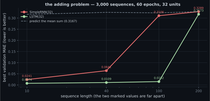
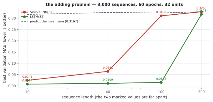
Two conclusions, and the second one matters more:

1. A SimpleRNN’s usable range ended between 40 and 100 timesteps here. That is why it scored 0.5856 on 200-token reviews — for most of each review it is not carrying anything.
2. The LSTM’s range is longer, not infinite. It won by a factor of twenty at 100 steps and then joined the SimpleRNN at the baseline at 200. Anyone who tells you gates “solve” long-range dependency should be asked at what length, with what budget.

sketch Unrolling the recurrence p5.js Pause Restart

Drag the recurrent weight and watch what the state does over 40 steps of identical input. Above 1 it explodes, below 1 it decays to a fixed point.

Drag the weight above 1 and the state pins at $\pm 1$; drop it below and the state collapses towards a single value. Neither extreme carries information forward, and the whole design of the LSTM is an answer to that.

sketch The measured table, ranked p5.js Pause Restart

Click a column to rank every row by it. The bars are that column's values and the highest and lowest are computed from the numbers, not written in.

Pitfalls

• Expecting a SimpleRNN to beat a bag of words on long text. Measured 0.5856 against 0.8004 on 200-token reviews.
• Forgetting return_sequences=True on a stacked layer. The next layer receives (batch, units) instead of (batch, timesteps, units) and either errors or silently treats units as timesteps.
• Post-padding a recurrent model. The output is the state after the padding; the state converges to a fixed point and the review is gone.
• Assuming the state is zero over padding. Measured mean |state| 0.2646 during padding against 0.2180 over the text — padding is not silence.
• Reading the parameter count as a function of sequence length. It is not: the same 2,080 parameters process 20 or 20,000 timesteps.
• Benchmarking against a shuffled control without checking the control. The bag-of-words model must score identically under shuffling; if it doesn’t, the shuffle is not doing what you think.
• Using tanh saturation as an explanation without measuring it. Here 0 of 32 units were saturated at the last step; the failure at long range is decay, not saturation.

Recap

• $h_t = \tanh(W_x x_t + W_h h_{t-1} + b)$, weights shared across timesteps, so the parameter count is independent of sequence length: 2,080 for SimpleRNN(32) on 32-dimensional inputs.
• The five-line NumPy version matches Keras to 5.96e-08 — the layer is exactly that loop.
• Order is worth +0.0744 to the RNN and, by construction, +0.0000 to a bag of words — which still beat the RNN 0.8004 to 0.5856.
• Over 132 steps of padding the state converges to a fixed point; mean |state| 0.2646 over padding against 0.2180 over the review.
• return_sequences=True returns every state and is mandatory for all but the last layer in a stack.
• On the adding problem the SimpleRNN worked at 10 and 40 steps (MAE 0.0241, 0.0641) and collapsed to the baseline at 100 (0.3106 against 0.3233); the LSTM held to 100 (0.0152) and failed at 200.

Next

The recurrent layer’s weakness is now measured rather than asserted. The gated cells that fix it — and the exact mechanism, recomputed from their own trained weights — are next: LSTM & GRU Networks.

pch.quizTag pch.quizDefaultTitle

1. A SimpleRNN(32) scored 0.5856 on IMDB while GlobalAveragePooling1D over the same embeddings scored 0.8004. What does that mean?

   A The RNN was implemented incorrectly B At 200 timesteps a plain recurrent state cannot carry information far enough to beat simply averaging the words — order helps (+0.0744) but the mechanism extracting it is too weak C Word order does not matter for sentiment D The bag-of-words model is cheating by seeing the labels
   pch.quizShowAnswer

   B — At 200 timesteps a plain recurrent state cannot carry information far enough to beat simply averaging the words — order helps (+0.0744) but the mechanism extracting it is too weak — The RNN's 0.0744 drop under shuffling proves it does use order. Gated cells are what make that usable at this length.

2. Why is the bag-of-words score identical (0.8004) in order and shuffled?

   A Because the shuffle failed B Because averaging is permutation-invariant — the pooled vector is mathematically the same however the tokens are ordered, which makes it the control for this experiment C Because both runs used the same random seed D Because the embedding layer sorts its input
   pch.quizShowAnswer

   B — Because averaging is permutation-invariant — the pooled vector is mathematically the same however the tokens are ordered, which makes it the control for this experiment — If that number had moved, the experiment would be broken. A control that must produce a known answer is worth including.

3. Over 132 steps of padding, the measured mean |state| was 0.2646 — higher than the 0.2180 over the real review. Why?

   A Because padding tokens have larger embeddings by design B Because token id 0 has an ordinary embedding vector, and feeding it repeatedly drives the recurrence to a fixed point h* = tanh(Wx·x_pad + Wh·h* + b) C Because the state accumulates without bound D Because tanh saturates at exactly 0.2646
   pch.quizShowAnswer

   B — Because token id 0 has an ordinary embedding vector, and feeding it repeatedly drives the recurrence to a fixed point h* = tanh(Wx·x_pad + Wh·h* + b) — That fixed point carries no information about the review, which is precisely why post-padding an unmasked RNN collapses to chance.

4. How many parameters does SimpleRNN(32) have on 32-dimensional inputs, and what does the sequence length change?

   A 2,080, and length changes nothing — the weights are shared across every timestep B 2,080 per timestep, so 200 timesteps means 416,000 C It depends on the batch size D 1,056, because the recurrent matrix is triangular
   pch.quizShowAnswer

   A — 2,080, and length changes nothing — the weights are shared across every timestep — 32*32 + 32*32 + 32 = 2,080. Weight sharing across time is what lets one layer handle any length.

5. When must you pass return_sequences=True?

   A Whenever the input is padded B When the next layer needs a sequence — stacking recurrent layers, per-timestep outputs, or attention. Every layer but the last in a stack requires it C Only for bidirectional layers D Whenever the batch size is greater than 1
   pch.quizShowAnswer

   B — When the next layer needs a sequence — stacking recurrent layers, per-timestep outputs, or attention. Every layer but the last in a stack requires it — Without it the layer emits (batch, units) and the following recurrent layer has no time axis to consume.

🧪 Try It Yourself

pch.exerciseTag pch.exerciseTitle

pch.exerciseTag pch.exerciseTitle

pch.exerciseTag pch.exerciseTitle

pch.exerciseTag pch.exerciseTitle

pch.exerciseTag pch.exerciseTitle