Pooling & CNN Architecture

Convolution keeps the resolution; something has to reduce it. The receptive-field arithmetic showed why: eight stride-1 layers see 17 pixels of a 28-pixel image, while downsampling reaches 511. This page measures the four ways of doing it, and one of the results contradicts the usual advice.

What you’ll learn

Pooling implemented by hand and matched to Keras at 0.00e+00 (max) and 5.96e−08 (average).
What each kind preserves: average pooling keeps the mean at 0.5761 exactly, max pooling raises it to 0.6738.
Four downsampling strategies measured, where average pooling (0.8740) matched max pooling (0.8720) and strided convolution came last at 0.8455.
What skipping downsampling costs: 14.7× the parameters and 3× the time for no reliable gain.
The activation-memory profile: 201,000 bytes per image, and where it goes.
Why Flatten before a Dense head is where a small convnet’s parameters disappear.

Pooling is a reduction with no parameters

Split the feature map into non-overlapping windows and replace each with one number — its maximum or its mean:

Both kinds, written out

def pool(image, size, how):
    blocks = image.reshape(image.shape[0] // size, size,
                           image.shape[1] // size, size)
    return blocks.max(axis=(1, 3)) if how == "max" else blocks.mean(axis=(1, 3))

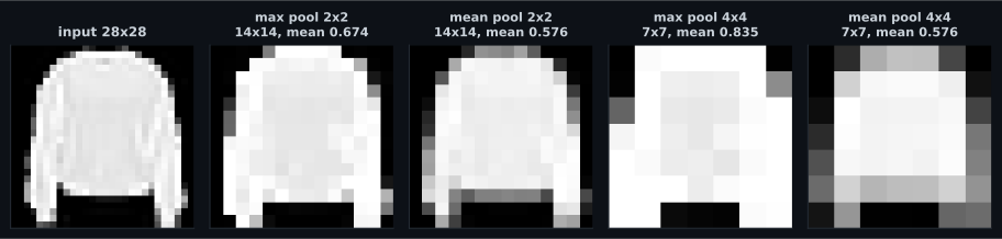
Matched against MaxPooling2D(2) and AveragePooling2D(2): maximum difference 0.00e+00 for max pooling and 5.96e−08 for average pooling — the latter is float32 rounding on the division. A 2×2 pool discards three of every four values: 784 numbers become 196.

Five greyscale panels: a 28x28 Fashion-MNIST pullover, then the same image after 2x2 max pooling and 2x2 average pooling at 14x14, and 4x4 max and average pooling at 7x7. The max-pooled versions look brighter and blockier; the average-pooled ones look softer. — Max pooling keeps the brightest pixel in each window, so the garment thickens and brightens — its mean rises from 0.5761 to 0.6738 at 2x2 and 0.8353 at 4x4. Average pooling preserves the mean exactly at 0.5761 in both cases, and loses the peaks instead: its maximum falls from 1.0000 to 0.9657 and then 0.9422.

	Output shape	Mean	Max	Std
input	(28, 28)	0.5761	1.0000	0.4329
max pool 2×2	(14, 14)	0.6738	1.0000	0.4185
average pool 2×2	(14, 14)	0.5761	0.9657	0.4008
max pool 4×4	(7, 7)	0.8353	1.0000	0.3229
average pool 4×4	(7, 7)	0.5761	0.9422	0.3450

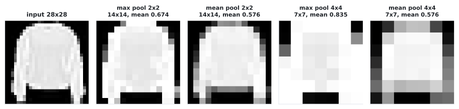
That table is the whole difference. Max pooling asks “did this feature appear anywhere in the window?” — it is a local OR, it keeps the peak, and it raises the mean because the maximum of four samples is above their average. Average pooling asks “how much of this feature was present on average?” — it preserves the mean by construction and destroys the peaks.

For a feature detector, the OR is usually what you want: a vertical edge somewhere in this 2×2 region is the useful fact. That is the standard argument for max pooling. The measurement below tests it.

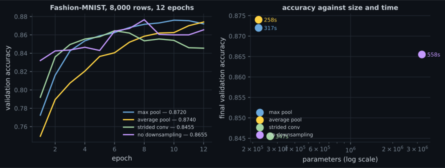
Four ways to halve the resolution

Same architecture, same seed, 8,000 Fashion-MNIST rows, 12 epochs — only the downsampling mechanism changes:

Two panels. Left: validation accuracy per epoch for four downsampling strategies, with max pool, average pool and no downsampling clustered near 0.87 and strided convolution below them. Right: a scatter of final accuracy against parameter count on a log axis, where no downsampling sits far to the right at 3.2 million parameters. — Max and average pooling are indistinguishable at 0.8720 and 0.8740 with identical parameter counts. Strided convolution adds 46,176 parameters and finishes last at 0.8455. Removing downsampling entirely reaches 0.8765 — the best 'best' figure — but needs 3,230,794 parameters and 345 seconds against max pooling's 220,234 and 116.

Strategy	Parameters	Final val accuracy	Best	Seconds
max pooling	220,234	0.8720	0.8760	116.3
average pooling	220,234	0.8740	0.8740	90.6
strided convolution	266,410	0.8455	0.8645	142.8
no downsampling	3,230,794	0.8655	0.8765	345.5

Three honest readings:

Average pooling matched max pooling. 0.8740 against 0.8720 final, with identical parameter counts, and average pooling was 22% faster in this run. The “max pooling is better for feature detection” argument is plausible and did not show up here. Both are fine; do not spend time choosing.
Strided convolution came last — 0.8455 — while adding 46,176 parameters and the most time of the three downsampling options. It is a learnable downsampler, which sounds better and here was worse.
Skipping downsampling was not the disaster the theory suggests. It reached the highest single number (0.8765), because it never throws information away. It also cost 14.7× the parameters and 3× the time, and those 3.2 million parameters are almost entirely in the Flatten → Dense transition, not in the convolutions.

The practical conclusion is the unglamorous one: pool with a 2×2 window, use max or average as you prefer, and spend the saved effort elsewhere.

The architecture that follows from this

diagram Diagram mermaid

  flowchart LR
  A["input
28x28x1"] --> B["Conv2D 32
28x28x32"]
  B --> C["MaxPool 2x2
14x14x32"]
  C --> D["Conv2D 64
14x14x64"]
  D --> E["MaxPool 2x2
7x7x64"]
  E --> F{"head"}
  F -- "Flatten" --> G["3,136 inputs
-> Dense 64"]
  F -- "GlobalAvgPool" --> H["64 inputs
-> Dense 64"]
  G --> I["Dense 10"]
  H --> I
  J["channels double as
resolution halves"] -.-> D

The pattern is almost universal: resolution halves and channel count doubles, so the total activation volume falls by 2× per block rather than 4×. Each block sees a larger region and represents more distinct patterns in it.

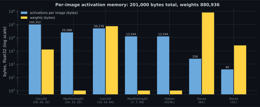
Where the memory actually goes

Training memory is dominated by stored activations, not weights — the backward pass needs every intermediate. Measured on the max-pool model:

figure Per-image activation memory against weight memory matplotlib

The two quantities are almost perfectly anti-correlated. The first convolution stores 100,352 bytes of activations from 1,280 bytes of weights; the Dense layer stores 256 bytes of activations from 803,072 bytes of weights. Total activations are 201,000 bytes per image, so a batch of 512 needs 102.91 MB before gradients are considered.

Layer	Output shape	Activations (bytes)	Weights (bytes)
Conv2D	(28, 28, 32)	100,352	1,280
MaxPooling2D	(14, 14, 32)	25,088	0
Conv2D	(14, 14, 64)	50,176	73,984
MaxPooling2D	(7, 7, 64)	12,544	0
Flatten	(3136,)	12,544	0
Dense	(64,)	256	803,072
Dense	(10,)	40	2,600

Batch size	Activation memory (forward only)
32	6.43 MB
128	25.73 MB
512	102.91 MB

Two things follow. Pooling early is the cheapest memory saving available — the first pool removes 75,264 bytes per image, more than every weight in the two convolutions combined. And the batch size you can fit is set by activations, which scale linearly with it, while weights do not scale at all.

The `Flatten` trap

Look again at that table: Dense(64) after Flatten holds 803,072 bytes of weights — 91% of the model’s parameters — because it receives $7 \times 7 \times 64 = 3{,}136$ inputs. Replace Flatten with GlobalAveragePooling2D and it receives 64.

Two heads, one of them enormous

keras.layers.Flatten(),                        # 3,136 inputs -> Dense(64)
keras.layers.GlobalAveragePooling2D(),         # 64 inputs -> Dense(64)

Global pooling averages each channel down to a single number, which discards position entirely. That is the right trade for classification — you want “a sleeve is present”, not “a sleeve is present at (3, 5)” — and it is why every architecture after VGG uses it.

sketch Pool a feature map by hand p5.js

A 8x8 map with a bright diagonal. Switch between max and average pooling at two window sizes and read what each one keeps.

sketch The measured table, ranked p5.js

Click a column to rank every row by it. The bars are that column's values and the highest and lowest are computed from the numbers, not written in.

Pitfalls

Believing max pooling is clearly better. Measured 0.8720 against average pooling’s 0.8740 with identical parameter counts.
Reaching for strided convolution because it is learnable. It finished last at 0.8455 and cost 46,176 extra parameters.
Using Flatten before the classifier head. It put 91% of this model’s parameters into one Dense layer. Use GlobalAveragePooling2D.
Budgeting memory from the parameter count. Activations dominate training memory and scale with the batch size; the first conv layer stored 78× more activation bytes than weight bytes.
Pooling too aggressively too early. A 4×4 pool on a 28-pixel image leaves 7×7 after one block; there is not much left to convolve.
Expecting pooling to add capacity. It has zero parameters and no nonlinearity. It buys receptive field and memory, nothing else.
Assuming no-downsampling is always worse. It reached the best single score here — at 14.7× the parameters and 3× the time.

Recap

Pooling replaces each window with its max or mean; max matched Keras at 0.00e+00 and average at 5.96e−08, and a 2×2 pool discards three of every four values.
Average pooling preserves the mean (0.5761 → 0.5761); max pooling raises it (→ 0.6738 at 2×2, 0.8353 at 4×4) and preserves the peaks.
Measured on 8,000 rows: average pool 0.8740, max pool 0.8720, no downsampling 0.8655 (best 0.8765 at 3.2M parameters), strided conv 0.8455.
The standard pattern is resolution halving while channels double, so activation volume falls 2× per block.
Activation memory is 201,000 bytes per image — 102.91 MB at batch 512 — and the first convolution holds half of it.
Flatten into Dense held 803,072 of 880,936 weight bytes. Global average pooling removes that at no measured cost in accuracy.

With convolution and downsampling settled, the interesting question is how to arrange them — and the answers that made history: Famous CNN Architectures (LeNet to ResNet).

pch.quizTag pch.quizDefaultTitle

Average pooling preserved the input's mean exactly (0.5761) while max pooling raised it to 0.6738. Why is that guaranteed rather than coincidental?

pch.quizShowAnswer

B — Because the mean of the window means is the mean of all values, while the maximum of four samples is at least their average and usually above it — This is also why max pooling keeps peaks and average pooling loses them: max 1.0000 against 0.9657 at 2x2.
Removing downsampling entirely gave the best single accuracy (0.8765) but needed 3,230,794 parameters against max pooling's 220,234. Where did the extra parameters come from?

pch.quizShowAnswer

B — From the Flatten to Dense transition: without pooling the final feature map is 28x28x64 = 50,176 values, so the Dense layer's kernel becomes enormous — That is also the Flatten trap in the pooled model, where Dense(64) held 91% of the parameters from 3,136 inputs.
Your convnet runs out of memory at batch 512 but fits at 128. What changed, given the weights are identical?

pch.quizShowAnswer

B — Activation memory scales linearly with the batch size — 25.73 MB at 128 against 102.91 MB at 512 here — while weight memory does not scale at all — And the backward pass needs every stored activation, so the real figure is higher than the forward-only number.
What does a MaxPooling2D layer contribute to a network?

pch.quizShowAnswer

B — Receptive field and reduced activation memory, and nothing else — it has zero parameters and applies no nonlinearity — It doubles the jump, which is what makes the receptive field grow geometrically rather than linearly with depth.
Strided convolution is a learnable downsampler, yet it scored 0.8455 against max pooling's 0.8720. What is the right takeaway?

pch.quizShowAnswer

B — A more flexible mechanism is not automatically better on a small dataset — it added 46,176 parameters to learn something a fixed rule already did well — On large datasets strided and learned downsampling do compete well. On 8,000 rows the fixed rule won, which is the general pattern for extra capacity on small data.

🧪 Try It Yourself

pch.coffeeTagline

pch.coffeeCta

pch.feedbackHeading

pch.feedbackSubheading