What you’ll learn

• why fitting the residual is gradient descent, taken in function space
• three boosting stages computed by hand, with the MSE at each one
• shrinkage measured: ten times smaller steps need roughly ten times more of them
• early stopping via staged_predictstaged_predict, and why it is not optional here
• how XGBoost, LightGBM and CatBoost actually differ, and when the difference matters
• an honest comparison where a boosted model does not win

Intuition

AdaBoost made the next learner focus on hard cases by reweighting the samples. Gradient boosting does the same thing with a change that turns out to be far more general: instead of reweighting, the next learner is fitted directly to what is left over.

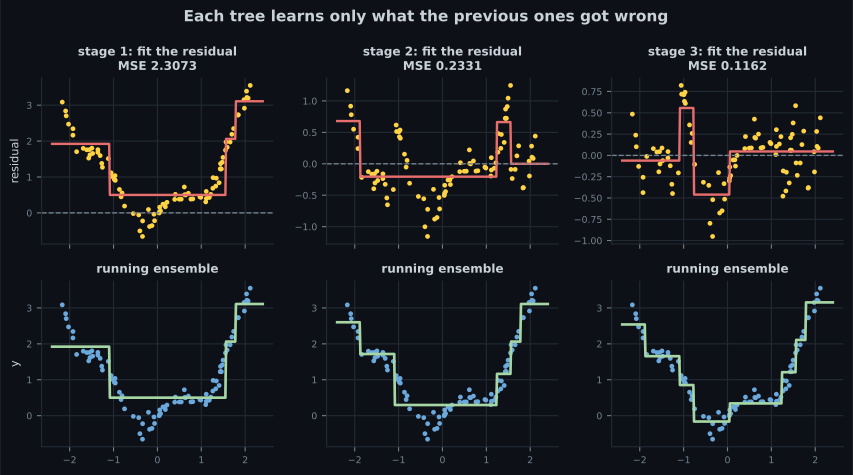
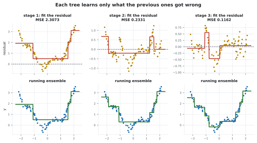
Predict the mean. Look at the residuals. Fit a small tree to the residuals. Add it. Look at the new residuals. Repeat.

That reframing is what lets gradient boosting handle any differentiable loss — squared error, absolute error, log loss, Poisson, quantile — with no change to the algorithm. AdaBoost’s reweighting turns out to be the special case for exponential loss.

  flowchart LR
  F0["F₀ = mean(y)"] --> R1["residual r₁ = y - F₀"]
  R1 --> H1["fit tree h₁ to r₁"]
  H1 --> F1["F₁ = F₀ + η·h₁"]
  F1 --> R2["residual r₂ = y - F₁"]
  R2 --> H2["fit tree h₂ to r₂"]
  H2 --> F2["F₂ = F₁ + η·h₂"]
  F2 --> D["... repeat"]

The math

Why the residual is a gradient

Take squared error as the loss for a single observation:

Differentiate with respect to the prediction $F$, not with respect to any parameter:

The residual is the negative gradient of the loss with respect to the prediction. So fitting a tree to the residuals is fitting a tree to the direction of steepest descent, and adding it is a gradient step:

Compare that with the parameter update from Gradient Descent Explained: $\boldsymbol{\theta} \leftarrow \boldsymbol{\theta} - \alpha\nabla J$. Same shape. The difference is that the step is a whole function rather than a parameter vector — hence “gradient descent in function space”.

The general algorithm

For any differentiable loss $L$:

1. $F_0(\mathbf{x}) = \arg\min_c \sum_i L(y_i, c)$ — the best constant.
2. For $m = 1, \ldots, M$:
   • compute pseudo-residuals $r_{im} = -\left[\partial L(y_i, F(\mathbf{x}_i)) / \partial F(\mathbf{x}_i)\right]_{F = F_{m-1}}$
   • fit a regression tree $h_m$ to the $r_{im}$
   • update $F_m = F_{m-1} + \eta\, h_m$

Swap the loss and only the pseudo-residual changes:

Notice the log-loss row: the pseudo-residual is $y - \sigma(F)$, exactly the gradient from logistic regression. The same expression appears for a third time, and for the same reason.

Worked example by hand

Three points: $x = [1, 2, 3]$, $y = [10, 20, 30]$. Learning rate $\eta = 0.5$, and each $h_m$ is a depth-1 stump.

Stage 0 — the constant. For squared error the best constant is the mean:

Stage 1 — fit the residuals. $r_1 = y - F_0 = [-10, 0, +10]$. A stump splitting at $x \le 1.5$ gives the left leaf $-10$ and the right leaf $\frac{0 + 10}{2} = 5$:

Stage 2 — fit those residuals. A stump splitting at $x \le 2.5$ gives the left leaf $\frac{-5 + (-2.5)}{2} = -3.75$ and the right leaf $7.5$:

Two things to notice. The predictions are walking toward $[10, 20, 30]$ without ever jumping there — that is $\eta = 0.5$ holding them back. And no individual stump is any good: the best of them predicts three distinct values. The ensemble is good; no member is.

figureThree stages on a curved datasetmatplotlib

See it move

Stage by stage, the ensemble grows toward the data while the residuals collapse toward zero.

Shrinkage

figureFour learning rates, 1200 trees eachmatplotlib

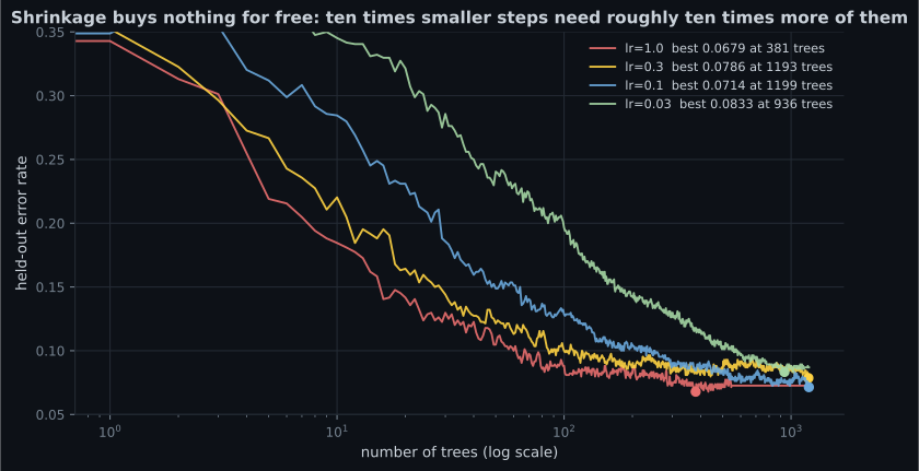
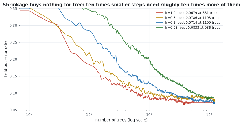
Measured on 1,560 held-out rows of the Hastie benchmark:

Reading the plot

1. Smaller learning rates need proportionally more trees. Roughly, $\eta \times M$ is conserved: 1.0 at 381 trees and 0.1 at 1,199 land within 0.4 points of each other.
2. They did not reach a lower floor here. The common claim that shrinkage always improves generalisation is not supported by this run — lr=1.0 was the best of the four. Shrinkage buys stability and control, not a guaranteed better score.
3. lr=0.03 has not converged at 1,200 trees. Its curve is still descending. Reporting it as “worse” would be reporting an unfinished experiment.
4. The practical rule survives: set a low learning rate, use early stopping to decide the tree count, and let the compute budget cap it. Just do not expect the low rate to pay for itself automatically.

Early stopping

n_estimatorsn_estimators in a boosted model can overfit, so it must be chosen rather than set. staged_predictstaged_predict replays the ensemble one tree at a time:

import numpy as np
from sklearn.datasets import make_hastie_10_2
from sklearn.ensemble import GradientBoostingClassifier
from sklearn.model_selection import train_test_split
 
X, y = make_hastie_10_2(n_samples=2400, random_state=0)
X_tr, X_te, y_tr, y_te = train_test_split(X, y, test_size=0.35, random_state=0)
 
model = GradientBoostingClassifier(n_estimators=1200, learning_rate=0.1,
                                   max_depth=3, random_state=0).fit(X_tr, y_tr)
 
errors = [1 - (pred == y_te).mean() for pred in model.staged_predict(X_te)]
best_n = int(np.argmin(errors)) + 1
 
print(f"best error {min(errors):.4f} at {best_n} trees")
print(f"error at 1200 trees {errors[-1]:.4f}")

import numpy as np
from sklearn.datasets import make_hastie_10_2
from sklearn.ensemble import GradientBoostingClassifier
from sklearn.model_selection import train_test_split
 
X, y = make_hastie_10_2(n_samples=2400, random_state=0)
X_tr, X_te, y_tr, y_te = train_test_split(X, y, test_size=0.35, random_state=0)
 
model = GradientBoostingClassifier(n_estimators=1200, learning_rate=0.1,
                                   max_depth=3, random_state=0).fit(X_tr, y_tr)
 
errors = [1 - (pred == y_te).mean() for pred in model.staged_predict(X_te)]
best_n = int(np.argmin(errors)) + 1
 
print(f"best error {min(errors):.4f} at {best_n} trees")
print(f"error at 1200 trees {errors[-1]:.4f}")

Or let scikit-learn stop for you, which avoids fitting trees you will discard:

GradientBoostingClassifier(
    n_estimators=2000,
    validation_fraction=0.15,     # hold out 15% internally
    n_iter_no_change=25,          # stop after 25 rounds without improvement
    tol=1e-4,
)

GradientBoostingClassifier(
    n_estimators=2000,
    validation_fraction=0.15,     # hold out 15% internally
    n_iter_no_change=25,          # stop after 25 rounds without improvement
    tol=1e-4,
)

HistGradientBoosting: the fast default

scikit-learn’s HistGradientBoosting*HistGradientBoosting* bins continuous features into 255 buckets before searching splits, which turns the split search from $O(m \log m)$ into $O(\text{bins})$. It is the same idea LightGBM introduced, and it is dramatically faster on anything over a few thousand rows.

from sklearn.datasets import load_breast_cancer
from sklearn.ensemble import (HistGradientBoostingClassifier,
                              RandomForestClassifier)
from sklearn.linear_model import LogisticRegression
from sklearn.model_selection import cross_val_score
from sklearn.pipeline import make_pipeline
from sklearn.preprocessing import StandardScaler
 
X, y = load_breast_cancer(return_X_y=True)
 
models = {
    "HistGradientBoosting": HistGradientBoostingClassifier(random_state=0),
    "RandomForest": RandomForestClassifier(n_estimators=200, random_state=0, n_jobs=-1),
    "LogisticRegression": make_pipeline(StandardScaler(),
                                        LogisticRegression(max_iter=5000)),
}
 
for name, model in models.items():
    print(f"{name:<22} CV {cross_val_score(model, X, y, cv=5).mean():.4f}")
 
# HistGradientBoosting   CV 0.9648
# RandomForest           CV 0.9596
# LogisticRegression     CV 0.9807

from sklearn.datasets import load_breast_cancer
from sklearn.ensemble import (HistGradientBoostingClassifier,
                              RandomForestClassifier)
from sklearn.linear_model import LogisticRegression
from sklearn.model_selection import cross_val_score
from sklearn.pipeline import make_pipeline
from sklearn.preprocessing import StandardScaler
 
X, y = load_breast_cancer(return_X_y=True)
 
models = {
    "HistGradientBoosting": HistGradientBoostingClassifier(random_state=0),
    "RandomForest": RandomForestClassifier(n_estimators=200, random_state=0, n_jobs=-1),
    "LogisticRegression": make_pipeline(StandardScaler(),
                                        LogisticRegression(max_iter=5000)),
}
 
for name, model in models.items():
    print(f"{name:<22} CV {cross_val_score(model, X, y, cv=5).mean():.4f}")
 
# HistGradientBoosting   CV 0.9648
# RandomForest           CV 0.9596
# LogisticRegression     CV 0.9807

HistGradientBoostingHistGradientBoosting also handles missing values natively — it learns which side of each split a NaN should go — so no imputer is required.

The four libraries

The differences that actually matter in practice:

• LightGBM grows leaf-wise: it splits whichever leaf reduces loss most, rather than completing each level. Deeper, more unbalanced trees, faster convergence — and easier overfitting on small data, so num_leavesnum_leaves needs care.
• CatBoost uses ordered target statistics for categorical features, which is target encoding done with a scheme that provably avoids the leakage a naive groupby().mean()groupby().mean() introduces. If your data is categorical-heavy, this is the reason to pick it.
• XGBoost adds explicit regularisation to the objective (lambdalambda, alphaalpha, gammagamma) and was the first to popularise the second-order (Newton) approximation of the loss.

Start with HistGradientBoostingHistGradientBoosting. No new dependency, competitive accuracy, and if it is not enough you now know what you are shopping for.

Pitfalls

Compare

🧪 Try It Yourself

Exercise 1 – The residual is the gradient

Exercise 2 – Two boosting stages by hand

Exercise 3 – Find the best number of trees

Exercise 4 – Run the cheap baseline first

Exercise 5 – Shrinkage trades against tree count

Recap

• The residual is the negative gradient of squared loss with respect to the prediction, so boosting is gradient descent in function space.
• Swapping the loss changes only the pseudo-residual, which is why gradient boosting handles log loss, Huber, quantile and Poisson with one algorithm.
• Hand-worked: MSE 66.667 → 29.167 → 8.073 in two stages, from stumps that individually predict two values each.
• Shrinkage trades against tree count roughly reciprocally — 1.0 peaked at 381 trees, 0.1 at 1,199 — and did not reach a lower floor in this run.
• n_estimatorsn_estimators can overfit. Use staged_predictstaged_predict or n_iter_no_changen_iter_no_change.
• Start with HistGradientBoostingHistGradientBoosting; reach for LightGBM on very large data and CatBoost on categorical-heavy data.
• Logistic regression beat both ensembles on breast cancer. Run the cheap baseline first.

Exercise 6 – Three boosting rounds, by hand

Next

Continue to Stacking and Voting Classifiers — the third family, where the members come from different algorithms entirely and a second-level model learns how much to trust each one.