Experiment Tracking and Reproducibility

What you’ll learn

how much of “my model gets 0.91” is the seed: range 0.0300 from the split alone
that sklearn is bit-reproducible when seeded — three runs, one hash: 25b525a8327c8ac025b525a8327c8ac0
the winner’s curse, measured: best-of-20 on 800 rows, validation-test correlation −0.0386
why paired comparison resolves a 0.0059 effect that unpaired comparison needs 26,000 rows for
what a run record must contain to be worth keeping, in about thirty lines
when to reach for MLflow or Weights & Biases, and when a JSONL file is genuinely enough

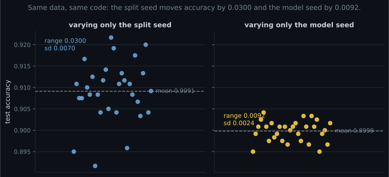
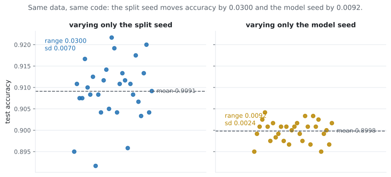
The number you reported is one of thirty

One dataset, one model, one script. Only the seed changes.

Two strip plots of test accuracy. Varying the split seed gives values from 0.8917 to 0.9217 with sd 0.0070. Varying the model seed gives 0.8950 to 0.9042 with sd 0.0024. — Thirty runs each. The train/test split contributes three times the spread of the model's own randomness, because it changes both what the model learns from and what it is measured on. A single run reports one dot from one of these clouds, and nothing about the cloud.

Source of randomness	Mean	sd	Min	Max	Range
train/test split seed	0.9091	0.0070	0.8917	0.9217	0.0300
model seed (fixed split)	0.8998	0.0024	0.8950	0.9042	0.0092

Three points follow, and the third is the one that matters.

Reporting one number is reporting a sample of size one. “0.9217” and “0.8917” are the same experiment. Neither is wrong; a claim built on either is.

The split dominates. Its sd is 2.9× the model seed’s, because a new split changes the training data and the test data. This is also why cross_val_scorecross_val_score reports a standard deviation — use it.

Any improvement smaller than 0.03 needs a protocol, not a run. If your new idea gains 0.01, a single comparison cannot see it. The rest of this page is about what to do instead.

Reproducibility is achievable, and it is not the hard part

Seed everything and sklearn is bit-identical. Not close — identical:

fingerprint.py

def fingerprint(model, X):
    """A hash of the predicted probabilities: identical runs, identical string."""
    proba = model.predict_proba(X)
    return hashlib.sha256(np.ascontiguousarray(proba).tobytes()).hexdigest()[:16]
 
 
for _ in range(3):
    print(fingerprint(RandomForestClassifier(n_estimators=200,
                                             random_state=0).fit(X_tr, y_tr), X_te))
# 25b525a8327c8ac0
# 25b525a8327c8ac0
# 25b525a8327c8ac0
 
# random_state=1 instead:
# 8458e21babe31fd5

fingerprint.py

def fingerprint(model, X):
    """A hash of the predicted probabilities: identical runs, identical string."""
    proba = model.predict_proba(X)
    return hashlib.sha256(np.ascontiguousarray(proba).tobytes()).hexdigest()[:16]
 
 
for _ in range(3):
    print(fingerprint(RandomForestClassifier(n_estimators=200,
                                             random_state=0).fit(X_tr, y_tr), X_te))
# 25b525a8327c8ac0
# 25b525a8327c8ac0
# 25b525a8327c8ac0
 
# random_state=1 instead:
# 8458e21babe31fd5

Three runs, one hash. So “I cannot reproduce my result” is almost never about the algorithm; it is about one of these:

What actually breaks reproducibility	How to fix it
The split was not seeded, or was re-drawn	`random_staterandom_state` on every splitter, recorded
The data changed under you	Hash the input file, or snapshot it
A library version changed	Record `pip freezepip freeze`, pin the important ones
Preprocessing depended on row order	Sort explicitly; never rely on a directory listing
A notebook was run out of order	Run the script end to end before believing it
GPU / thread nondeterminism	Real for deep learning; not for the sklearn code above

The fingerprint above is worth adopting as a habit. Print it at the end of training and paste it into the run record: two runs that claim to be the same and hash differently are not the same, and you find out in one second instead of one week.

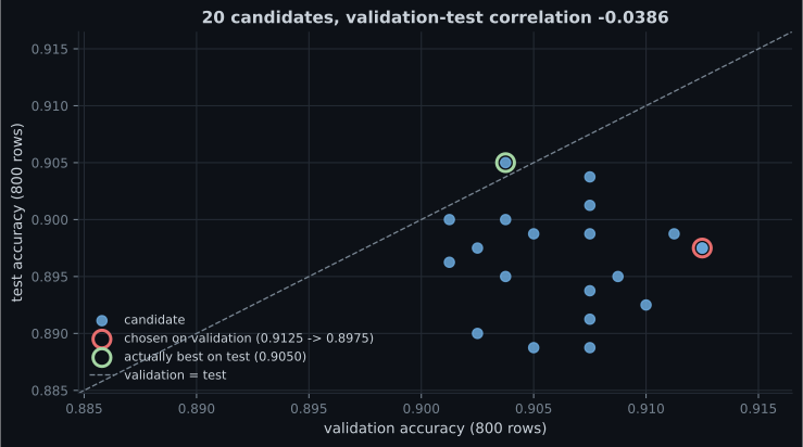
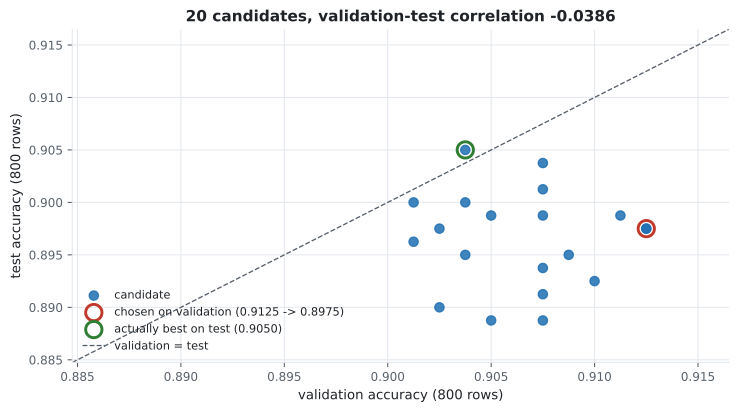
The winner’s curse

Here is the mistake that survives even a careful reproducibility setup. Twenty candidate configurations, one validation set of 800 rows, pick the best.

Scatter of test accuracy against validation accuracy for 20 candidates, forming a shapeless cloud. The candidate with the highest validation accuracy, 0.9125, has test accuracy 0.8975, while the best test candidate at 0.9050 was middling on validation. — The cloud has no slope. Selecting on 800 validation rows selected noise: the validation winner (0.9125) came 13th on test (0.8975), while the genuinely best candidate (0.9050) was unremarkable on validation. The optimism of the selected number is +0.0150 — and reporting the validation score of the selected model is the standard way to overstate a result.

	Value
best validation accuracy	0.9125 (candidate 2)
that candidate’s test accuracy	0.8975
selection optimism	+0.0150
best test accuracy available	0.9050 (candidate 11)
validation-test correlation	−0.0386

The mechanism is arithmetic. Accuracy on 800 rows near 0.906 has a binomial standard error of

\mathrm{se} = \sqrt{\frac{p(1-p)}{n}} = \sqrt{\frac{0.906 \times 0.094}{800}} = 0.0103

so two independent estimates of the same underlying accuracy differ by up to $1.96\sqrt{2} \times 0.0103 = 0.0286$ purely by chance. The 20 candidates differ genuinely by far less than that. Taking a maximum over 20 draws from that noise gives you the noisiest candidate, not the best one.

To resolve a 0.005 difference between two independent measurements at this accuracy you would need

n = \frac{\big(1.96\sqrt{2}\big)^2 \, p(1-p)}{0.005^2} \approx 26{,}173 \text{ rows}

Which you do not have. Fortunately, you do not need them.

See it move

One run of 20 candidates is an anecdote. The sketch runs the whole experiment repeatedly: candidates whose true accuracies differ only slightly, scored on 800 validation rows and 2,000 test rows, with the validation winner selected each time. The bars are the accumulated averages, so the bias is visible as a stable quantity rather than a story about one unlucky draw.

sketch Selection optimism grows with the number of candidates p5.js

Repeated experiments in which candidates with nearly identical true accuracy are scored on 800 validation rows and 2,000 test rows. The validation winner's validation score is consistently higher than its test score, and the gap grows as more candidates are compared. Click to step the candidate count.

The same simulation in NumPy, 20,000 experiments per row, so the sketch’s drifting averages can be checked against settled ones:

Candidates compared	Mean selection optimism	Mean shortfall vs the best candidate
2	+0.0054	−0.0035
5	+0.0109	−0.0071
10	+0.0144	−0.0093
20	+0.0174	−0.0114
50	+0.0207	−0.0136
100	+0.0230	−0.0150

The measured optimism at 20 candidates, +0.0174, is close to the +0.0150 seen in the single run above — that run was ordinary, not unlucky. Two consequences follow directly. The bias grows with the number of things you compare, so a hyperparameter sweep of 100 trials inflates its own headline by roughly 0.023 on this problem. And the second column says the cost is not only in the reporting: the model you ship is on average 0.011 worse than the best one you actually trained, because validation noise picked the wrong candidate.

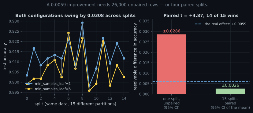
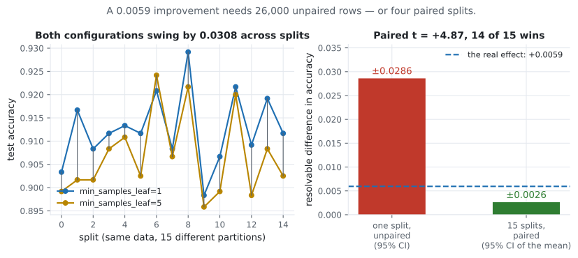
Pair your comparisons

The variance above comes almost entirely from which rows landed in the test set — and that variance is shared if you evaluate both candidates on the same splits. Subtract, and it cancels.

Left: two configurations' accuracy across 15 identical splits, tracking each other closely with min_samples_leaf=1 above min_samples_leaf=5 on almost every split. Right: resolvable difference — plus or minus 0.0286 for one unpaired split against plus or minus 0.0026 for 15 paired splits, with the real 0.0059 effect marked. — Both configurations swing by 0.0308 across splits, so either one alone tells you nothing. But they swing together: the difference has a standard deviation of only 0.0047, giving a paired t of +4.87 and 14 wins out of 15. The effect was always there; the unpaired protocol simply could not see it.

paired_comparison.py

a, b = [], []
for s in range(15):
    X_tr, X_te, y_tr, y_te = train_test_split(X, y, test_size=0.3,
                                              random_state=100 + s, stratify=y)
    a.append(score(config_a, X_tr, y_tr, X_te, y_te))     # same split
    b.append(score(config_b, X_tr, y_tr, X_te, y_te))     # for both
 
diff = np.array(a) - np.array(b)
t = diff.mean() / (diff.std(ddof=1) / np.sqrt(len(diff)))
print(f"{diff.mean():+.4f} +- {diff.std(ddof=1):.4f}   t {t:+.2f}   "
      f"{(diff > 0).sum()} of {len(diff)} wins")
# +0.0059 +- 0.0047   t +4.87   14 of 15 wins

paired_comparison.py

a, b = [], []
for s in range(15):
    X_tr, X_te, y_tr, y_te = train_test_split(X, y, test_size=0.3,
                                              random_state=100 + s, stratify=y)
    a.append(score(config_a, X_tr, y_tr, X_te, y_te))     # same split
    b.append(score(config_b, X_tr, y_tr, X_te, y_te))     # for both
 
diff = np.array(a) - np.array(b)
t = diff.mean() / (diff.std(ddof=1) / np.sqrt(len(diff)))
print(f"{diff.mean():+.4f} +- {diff.std(ddof=1):.4f}   t {t:+.2f}   "
      f"{(diff > 0).sum()} of {len(diff)} wins")
# +0.0059 +- 0.0047   t +4.87   14 of 15 wins

Protocol	Resolvable difference (95%)
one split, two independent numbers	±0.0286
15 paired splits, CI of the mean difference	±0.0026
the actual effect	+0.0059

Four paired splits would have been enough: $(2.145 \times 0.0047 / 0.005)^2 = 4.1$ . The same comparison, done unpaired on one split, needs a test set 30× larger than the one available.

Practical form of the rule: cross_val_scorecross_val_score with the same cvcv object for both candidates, then compare fold by fold. The paired structure is what makes cross-validation a comparison tool rather than just a variance estimate. And report the win count alongside the mean — 14 of 15 is more persuasive to a sceptical reader than any p-value.

What a run record has to contain

The minimum that makes a result re-derivable a year later, in one file per project:

tracker.py

"""A run log that is a JSONL file. No server, no SDK, no account."""
 
import hashlib
import json
import platform
import subprocess
import time
from pathlib import Path
 
LOG = Path("runs.jsonl")
 
 
def config_hash(config: dict) -> str:
    """Order-independent identity for a configuration."""
    payload = json.dumps(config, sort_keys=True, separators=(",", ":"))
    return hashlib.sha256(payload.encode()).hexdigest()[:12]
 
 
def git_commit() -> str:
    try:
        out = subprocess.run(["git", "rev-parse", "--short", "HEAD"],
                             capture_output=True, text=True, check=True)
        dirty = subprocess.run(["git", "status", "--porcelain"],
                               capture_output=True, text=True, check=True)
        return out.stdout.strip() + ("-dirty" if dirty.stdout.strip() else "")
    except Exception:
        return "no-git"
 
 
def log_run(config: dict, metrics: dict, data_fingerprint: str,
            predictions_hash: str, notes: str = "") -> dict:
    import numpy, sklearn
 
    record = {
        "run_id": config_hash(config),
        "logged_at": time.strftime("%Y-%m-%dT%H:%M:%S"),
        "git": git_commit(),
        "config": config,
        "metrics": metrics,
        "data": data_fingerprint,
        "predictions_sha": predictions_hash,
        "env": {"python": platform.python_version(),
                "numpy": numpy.__version__,
                "sklearn": sklearn.__version__},
        "notes": notes,
    }
    with LOG.open("a", encoding="utf-8") as fh:
        fh.write(json.dumps(record, sort_keys=True) + "\n")
    return record

tracker.py

"""A run log that is a JSONL file. No server, no SDK, no account."""
 
import hashlib
import json
import platform
import subprocess
import time
from pathlib import Path
 
LOG = Path("runs.jsonl")
 
 
def config_hash(config: dict) -> str:
    """Order-independent identity for a configuration."""
    payload = json.dumps(config, sort_keys=True, separators=(",", ":"))
    return hashlib.sha256(payload.encode()).hexdigest()[:12]
 
 
def git_commit() -> str:
    try:
        out = subprocess.run(["git", "rev-parse", "--short", "HEAD"],
                             capture_output=True, text=True, check=True)
        dirty = subprocess.run(["git", "status", "--porcelain"],
                               capture_output=True, text=True, check=True)
        return out.stdout.strip() + ("-dirty" if dirty.stdout.strip() else "")
    except Exception:
        return "no-git"
 
 
def log_run(config: dict, metrics: dict, data_fingerprint: str,
            predictions_hash: str, notes: str = "") -> dict:
    import numpy, sklearn
 
    record = {
        "run_id": config_hash(config),
        "logged_at": time.strftime("%Y-%m-%dT%H:%M:%S"),
        "git": git_commit(),
        "config": config,
        "metrics": metrics,
        "data": data_fingerprint,
        "predictions_sha": predictions_hash,
        "env": {"python": platform.python_version(),
                "numpy": numpy.__version__,
                "sklearn": sklearn.__version__},
        "notes": notes,
    }
    with LOG.open("a", encoding="utf-8") as fh:
        fh.write(json.dumps(record, sort_keys=True) + "\n")
    return record

Eight fields, and each one exists because its absence has cost somebody a week:

Field	The question it answers later
`run_idrun_id` (config hash)	Have I already run exactly this?
`gitgit` (with `-dirty-dirty`)	Which code produced it — and was the tree clean?
`configconfig`	Every value that was a choice, including the seeds
`metricsmetrics`	All of them, not just the one that looked good
`datadata`	Which snapshot of the data — a hash or a version string
`predictions_shapredictions_sha`	Is this genuinely the same run as that one?
`envenv`	Which library versions
`notesnotes`	Why you tried it, in one sentence

The hash is order-independent and change-sensitive, which is exactly what you want from an identity:

identity.py

config = {"model": "random_forest", "n_estimators": 200,
          "min_samples_leaf": 1, "split_seed": 0, "model_seed": 0}
 
print(config_hash(config))                                    # 4894b21f75a6
print(config_hash({k: config[k] for k in reversed(config)}))   # 4894b21f75a6
print(config_hash({**config, "min_samples_leaf": 5}))          # b5e5037ae938

identity.py

config = {"model": "random_forest", "n_estimators": 200,
          "min_samples_leaf": 1, "split_seed": 0, "model_seed": 0}
 
print(config_hash(config))                                    # 4894b21f75a6
print(config_hash({k: config[k] for k in reversed(config)}))   # 4894b21f75a6
print(config_hash({**config, "min_samples_leaf": 5}))          # b5e5037ae938

The workflow

diagram Diagram mermaid

  flowchart TD
  A["An idea"] --> B["Write the config as data,
seeds included"]
  B --> C{"Has this run_id
been logged?"}
  C -->|"yes"| D["Read the metrics.
Do not rerun."]
  C -->|"no"| E["Train once.
Log config, metrics, env,
data hash, prediction hash."]
  E --> F{"Comparing against
another config?"}
  F -->|"yes"| G["Evaluate BOTH on the
same splits. Report the paired
mean, sd and win count."]
  F -->|"no"| H["Report the metric with
its cross-validated sd"]
  G --> I{"Effect bigger than
the paired CI?"}
  I -->|"no"| J["No measurable difference.
Say so, and keep the
simpler model."]
  I -->|"yes"| K["Confirm ONCE on the
untouched test set.
That number is the result."]
  H --> K

Pitfalls

Pitfall	Why it bites	What to do
Reporting one run’s accuracy	The split seed alone spans 0.0300	Report cross-validated mean and sd
Reporting the selection score	Optimism was +0.0150 over 20 candidates	Keep a test set for one final measurement
Comparing candidates unpaired	Needs 26,000 rows to resolve 0.0059	Same `cvcv` object for both; compare fold by fold
Tuning hundreds of configurations on a small validation set	Validation-test correlation was −0.0386	Fewer, better-motivated candidates; nested CV if you must search
Trusting “same code, same result”	An unrecorded seed or data version breaks it silently	Hash the predictions and compare the hashes
Logging only the winning metric	You cannot tell later whether a run was worse or just different	Log every metric you computed
A dirty git tree at training time	The commit does not describe the code that ran	Record `-dirty-dirty` and refuse to promote such runs
Notebook-only experiments	Out-of-order execution is unreproducible by construction	Run the script top to bottom before believing the number

Recap

Varying only the split seed moved test accuracy across 0.8917 → 0.9217 (sd 0.0070); the model seed moved it 0.0092.
Seeded sklearn is bit-reproducible: three runs, one prediction hash 25b525a8327c8ac025b525a8327c8ac0.
Best-of-20 on 800 validation rows: 0.9125 validation, 0.8975 test, optimism +0.0150, validation-test correlation −0.0386.
Unpaired resolution at this accuracy is ±0.0286; the real effect was +0.0059.
Paired over 15 splits: +0.0059 ± 0.0047, t +4.87, 14 of 15 wins — and four splits would have sufficed.
A useful run record has eight fields; a JSONL file with all eight beats a tracking server with six.

quizCheck yourself

You report test accuracy 0.9217. A colleague reruns your script and gets 0.8917. Who is wrong?
Show answer
B — Neither: the train/test split seed alone spans that range on this data, and a single run is a sample of size one — Measured range across 30 split seeds was exactly 0.8917 to 0.9217. Report a cross-validated mean with its standard deviation, and record the seed so the specific number is at least re-derivable.
Three runs of your seeded script produce three different prediction hashes. What does that mean?
Show answer
B — Something is unseeded or changing between runs — seeded sklearn is bit-identical, so identical hashes are the expectation — The measured case gave 25b525a8327c8ac0 three times in a row. Differing hashes point at an unseeded splitter, changing input data, or a library difference — and the hash finds it in a second rather than a week.
You tried 20 configurations, the best scored 0.9125 on validation, and you report that. What is wrong?
Show answer
B — Two things: the validation set that selected the model cannot estimate it (+0.0150 optimism here), and on 800 rows the selection was essentially random (correlation -0.0386) — The maximum over 20 noisy draws is a measurement of the noise. Keep an untouched test set for the final number, and reduce the number of comparisons — searching harder makes the reported number worse, not better.
Your new configuration looks 0.006 better. How do you establish that in the data you have?
Show answer
B — Evaluate both configurations on the same 15 splits and test the paired difference — it gave +0.0059 ± 0.0047, t = +4.87, 14 of 15 wins — Pairing cancels the split-to-split variance that dominates the unpaired comparison. The same effect that needs 26,000 unpaired rows becomes clear with four paired splits — and the win count communicates it more honestly than a p-value.
Which single field is most often missing from a run record, and most expensive to lack?
Show answer
B — The data snapshot identity — a hash or version of the input, without which no result can be re-derived even with perfect code and seeds — Code and seeds are usually recoverable from git; the data as it was on that day usually is not. A hash of the input file, or a dataset version string, is the field that keeps a result alive.

🧪 Try It Yourself

Exercise 1 – Measure your own noise floor

Exercise 2 – Fingerprint a model

Exercise 3 – Reproduce the winner’s curse

Exercise 4 – Pair the comparison

Exercise 5 – Build the run record

Data Validation and Schema Contracts — reproducing your own run is the easy half. The other half is noticing when the data underneath it changes shape, and the measured cost of not noticing.

If this helped you, consider buying me a coffee ☕

Buy me a coffee