Lengths and Distances

An inner product hands you two things immediately and for free. Length is the inner product of a vector with itself, square-rooted. Distance is the length of a difference. Both definitions are one line long, and between them they underpin every nearest-neighbour query, every clustering algorithm and every loss function you will meet.

The free part deserves emphasis. You do not choose a norm and a distance separately from an inner product — once the inner product is fixed, both are determined. Which means a change of inner product silently changes what “close” means, and this page ends by measuring exactly how much.

What you’ll learn

• The induced norm, and the fact that every inner product gives a norm while not every norm comes from an inner product.
• The Cauchy-Schwarz inequality, why it is the thing that makes the cosine of an angle well defined, and when it holds with equality.
• The definition of a metric and its three axioms, and how they line up with the norm axioms.
• The book’s Remark that an inner product and a metric behave in opposite directions — and why that is not a curiosity.
• The measured demonstration that $\ell_1$, $\ell_2$, $\ell_\infty$ and Mahalanobis distance disagree about which of nine candidates is nearest.

Intuition: the ruler is built into the tape measure

Suppose someone hands you a device that, given two directions, reports how much they overlap. You can build a ruler out of it without asking for anything else: to measure a stick, ask the device how much the stick overlaps with itself. A long stick overlaps itself a lot.

That is exactly what the induced norm does, and the square root is there for the reason you would expect — overlap-with-self scales with the square of length (an inner product is bilinear, so doubling the vector quadruples the answer), so you take a square root to get back to something that scales linearly.

Distance is then a second free step: the distance between two points is the length of the arrow from one to the other.

diagram Diagram mermaid

  flowchart TD
  IP["⟨x, y⟩
an inner product"]
  IP --> NORM["‖x‖ = √⟨x,x⟩
the INDUCED norm, Eq 3.16"]
  NORM --> DIST["d(x,y) = ‖x − y‖ = √⟨x−y, x−y⟩
a METRIC, Def 3.6"]
  IP --> CS["Cauchy-Schwarz
|⟨x,y⟩| ≤ ‖x‖ ‖y‖
Eq 3.17"]
  CS --> COS["so ⟨x,y⟩/(‖x‖‖y‖) lies in [−1, 1]
and can be a cosine — §3.4"]
  NORM --> ONEWAY["every inner product gives a norm
NOT every norm comes from one
(l1 and l-infinity do not)"]
  DIST --> AXIOMS["positive definite · symmetric · triangle inequality"]

The bottom-left node is the asymmetry to remember. Inner products are a strictly smaller world than norms. The $\ell_1$ and $\ell_\infty$ norms of the previous page are genuine norms that no inner product produces — which is why $\ell_1$ has no notion of angle attached to it and $\ell_2$ does.

The math

The induced norm

Equation 3.16 — the induced norm

Every inner product induces a norm:

$$\lVert \mathbf{x} \rVert := \sqrt{\langle \mathbf{x}, \mathbf{x}\rangle}$$

This is well defined precisely because the inner product is positive definite: the quantity under the root is positive for every nonzero $\mathbf{x}$ and zero only for $\mathbf{x} = \mathbf{0}$.

Check the three norm axioms against it and each one comes from an inner product property:

norm axiom	comes from
$\lVert\lambda\mathbf{x}\rVert = \lvert\lambda\rvert\lVert\mathbf{x}\rVert$	bilinearity: $\langle\lambda\mathbf{x},\lambda\mathbf{x}\rangle = \lambda^2\langle\mathbf{x},\mathbf{x}\rangle$, then the square root
$\lVert\mathbf{x}\rVert \geq 0$, zero only at $\mathbf{0}$	positive definiteness, directly
$\lVert\mathbf{x}+\mathbf{y}\rVert \leq \lVert\mathbf{x}\rVert + \lVert\mathbf{y}\rVert$	Cauchy-Schwarz — see below

The third one is not automatic, and Cauchy-Schwarz is exactly the tool that supplies it.

Cauchy-Schwarz

Equation 3.17 — Cauchy-Schwarz inequality

For an inner product vector space $(V, \langle\cdot,\cdot\rangle)$, the induced norm satisfies

$$\lvert \langle \mathbf{x}, \mathbf{y}\rangle \rvert \;\leq\; \lVert\mathbf{x}\rVert\,\lVert\mathbf{y}\rVert$$

with equality if and only if $\mathbf{x}$ and $\mathbf{y}$ are parallel — that is, one is a scalar multiple of the other.

Two consequences, and both matter.

It makes the cosine possible. Dividing through gives

$$-1 \;\leq\; \frac{\langle\mathbf{x},\mathbf{y}\rangle}{\lVert\mathbf{x}\rVert\,\lVert\mathbf{y}\rVert} \;\leq\; 1$$

and a number guaranteed to lie in $[-1,1]$ is a number you are allowed to call $\cos\omega$. Without Cauchy-Schwarz, $\arccos$ of that ratio might not exist and §3.4 would have nothing to define.

It gives the triangle inequality. Expand and bound:

$$\lVert\mathbf{x}+\mathbf{y}\rVert^2 = \langle\mathbf{x},\mathbf{x}\rangle + 2\langle\mathbf{x},\mathbf{y}\rangle + \langle\mathbf{y},\mathbf{y}\rangle \;\leq\; \lVert\mathbf{x}\rVert^2 + 2\lVert\mathbf{x}\rVert\lVert\mathbf{y}\rVert + \lVert\mathbf{y}\rVert^2 = \big(\lVert\mathbf{x}\rVert + \lVert\mathbf{y}\rVert\big)^2$$

The single inequality step replaces $\langle\mathbf{x},\mathbf{y}\rangle$ by $\lVert\mathbf{x}\rVert\lVert\mathbf{y}\rVert$, which is Cauchy-Schwarz, and taking square roots finishes it.

Distance and metrics

Definition 3.6 — Distance and metric

For an inner product space $(V, \langle\cdot,\cdot\rangle)$, the distance between $\mathbf{x}, \mathbf{y} \in V$ is

$$d(\mathbf{x}, \mathbf{y}) := \lVert \mathbf{x} - \mathbf{y}\rVert = \sqrt{\langle \mathbf{x}-\mathbf{y},\ \mathbf{x}-\mathbf{y}\rangle}$$

If the inner product is the dot product this is the Euclidean distance. The mapping

$$d : V \times V \to \mathbb{R}, \qquad (\mathbf{x},\mathbf{y}) \mapsto d(\mathbf{x},\mathbf{y})$$

is called a metric, and satisfies:

axiom	statement
positive definite	$d(\mathbf{x},\mathbf{y}) \geq 0$, and $d(\mathbf{x},\mathbf{y}) = 0 \iff \mathbf{x} = \mathbf{y}$
symmetric	$d(\mathbf{x},\mathbf{y}) = d(\mathbf{y},\mathbf{x})$
triangle inequality	$d(\mathbf{x},\mathbf{z}) \leq d(\mathbf{x},\mathbf{y}) + d(\mathbf{y},\mathbf{z})$

Note that a metric needs only these three. It does not need to come from a norm, let alone from an inner product — edit distance on strings and shortest-path distance on a graph are metrics with no vectors in sight. The hierarchy runs one way:

$$\text{inner products} \subset \text{norms} \subset \text{metrics}$$

The remark worth pausing on

The book adds a Remark that the inner product and the metric behave in opposite directions. Two vectors that are similar have a large inner product and a small distance; two that are dissimilar have a small inner product and a large distance.

This is not a curiosity, it is a recurring source of sign errors. A similarity has to be negated or inverted to be used as a distance, and code that treats an inner product as a distance will confidently return the farthest point when asked for the nearest. Note also that the correspondence is not a simple negation — expanding

$$\lVert\mathbf{x}-\mathbf{y}\rVert^2 = \lVert\mathbf{x}\rVert^2 - 2\langle\mathbf{x},\mathbf{y}\rangle + \lVert\mathbf{y}\rVert^2$$

shows that the distance depends on the inner product and on both lengths. Ranking by inner product and ranking by distance agree only when all the vectors have the same length, which is exactly the normalisation that turns a dot product into a cosine.

From the book

Section 3.3. The induced norm is Equation 3.16 and Cauchy-Schwarz Equation 3.17. Example 3.5 (Equations 3.18 to 3.20) measures $\mathbf{x} = (1,1)^\top$ under two different inner products. Definition 3.6 gives distance and metric (Equation 3.21), with Equations 3.22 and 3.23 for the symmetry and triangle-inequality properties. The Remark about inner products and metrics behaving in opposite directions closes the section.

Worked example by hand

Example 3.5 from the book

Take $\mathbf{x} = (1,1)^\top \in \mathbb{R}^2$. Under the dot product:

$$\lVert\mathbf{x}\rVert = \sqrt{\mathbf{x}^\top\mathbf{x}} = \sqrt{1^2 + 1^2} = \sqrt{2} \approx 1.414214$$

Now take instead the inner product of the book’s Equation 3.19,

$$\langle\mathbf{x},\mathbf{y}\rangle := \mathbf{x}^\top\begin{bmatrix} 1 & -\frac{1}{2} \\ -\frac{1}{2} & 1\end{bmatrix}\mathbf{y} = x_1y_1 - \tfrac{1}{2}\left(x_1y_2 + x_2y_1\right) + x_2y_2$$

and the same vector measures

$$\lVert\mathbf{x}\rVert = \sqrt{1 - \tfrac{1}{2}(1 + 1) + 1} = \sqrt{1 - 1 + 1} = \sqrt{1} = 1 .$$

Exactly $1$, not approximately. The book’s phrasing is that this inner product makes us “perceive” $\mathbf{x}$ as shorter than the dot product does. The reason is the negative off-diagonal entry: it subtracts a penalty proportional to $x_1x_2$, so vectors whose coordinates agree in sign are discounted. Under this inner product, $(1,1)$ is a unit vector.

The book’s Exercise 3.3, worked

Compute the distance between $\mathbf{x} = (1,2,3)^\top$ and $\mathbf{y} = (-1,-1,0)^\top$ under two inner products. First the difference:

$$\mathbf{x} - \mathbf{y} = (2,\ 3,\ 3)^\top$$

(a) Dot product. $\lVert(2,3,3)\rVert^2 = 4 + 9 + 9 = 22$, so $d = \sqrt{22} \approx 4.690416$.

(b) With $\mathbf{A} = \begin{bmatrix} 2&1&0\\1&3&-1\\0&-1&2\end{bmatrix}$. First $\mathbf{A}(\mathbf{x}-\mathbf{y})$, row by row:

row	working	result
1	$2(2) + 1(3) + 0(3)$	$7$
2	$1(2) + 3(3) + (-1)(3)$	$8$
3	$0(2) + (-1)(3) + 2(3)$	$3$

Then $(2,3,3)\cdot(7,8,3) = 14 + 24 + 9 = 47$, so $d = \sqrt{47} \approx 6.855655$.

The second answer is larger, and $\mathbf{A}$ is a valid inner product: its eigenvalues are exactly $1$, $2$ and $4$. So the same two points are $4.69$ apart under one geometry and $6.86$ apart under another, and neither number is wrong.

worked_examples.py

import numpy as np
 
# Example 3.5
x = np.array([1.0, 1.0])
E = np.array([[1.0, -0.5], [-0.5, 1.0]])
print("Example 3.5:  dot", np.sqrt(x @ x), " Eq 3.19", np.sqrt(x @ E @ x))
 
# Exercise 3.3
p = np.array([1.0, 2.0, 3.0])
q = np.array([-1.0, -1.0, 0.0])
d = p - q
A = np.array([[2.0, 1.0, 0.0], [1.0, 3.0, -1.0], [0.0, -1.0, 2.0]])
print("difference:", d)
print("A @ d     :", A @ d)
print("(a) dot   :", float(d @ d), "->", np.sqrt(float(d @ d)))
print("(b) A form:", float(d @ A @ d), "->", np.sqrt(float(d @ A @ d)))
print("A eigenvalues:", np.round(np.linalg.eigvalsh(A), 6),
      " spd:", bool(np.all(np.linalg.eigvalsh(A) > 0)))

output

Example 3.5:  dot 1.4142135623730951  Eq 3.19 1.0
difference: [2. 3. 3.]
A @ d     : [7. 8. 3.]
(a) dot   : 22.0 -> 4.69041575982343
(b) A form: 47.0 -> 6.855654600401044
A eigenvalues: [1. 2. 4.]  spd: True

See it move

The first sketch tests the triangle inequality by hand. Drag the waypoint and watch the detour bar; it never falls below the direct bar, and it touches it exactly when the waypoint lies on the straight segment.

sketch A detour is never a shortcut p5.js Pause Restart

Drag the waypoint y between the fixed endpoints x and z. The bars compare the direct distance with the detour through y. Use the metric knob to switch between l1, l2 and the maximum norm; the inequality holds for all three, but for l1 and l-infinity the set of waypoints achieving equality is much larger than the straight segment.

The second sketch is Example 3.5, made draggable. Two inner products, two unit sets, one vector, two lengths.

sketch Example 3.5: one vector, two lengths p5.js Pause Restart

Drag x. The blue circle is the set of vectors the dot product calls unit length; the amber ellipse is the set Equation 3.19 calls unit length. The two readouts are the two lengths of the same arrow. At x = (1, 1) the amber value is exactly 1, which is the book's example.

The third makes Cauchy-Schwarz into a bar you can try to break. You cannot.

sketch Cauchy-Schwarz, as a bar you cannot overfill p5.js Pause Restart

Drag either arrow. The blue bar is the absolute inner product and the grey bar behind it is the product of the two lengths. The blue bar can reach the grey one but never pass it, and the ratio of the two is exactly the absolute cosine of the angle — which is the subject of the next page.

From scratch

metrics_from_scratch.py

import numpy as np
 
def induced_norm(x, A=None):
    """sqrt(<x,x>). A=None means the dot product."""
    q = x @ x if A is None else x @ A @ x
    return np.sqrt(q)
 
def induced_distance(x, y, A=None):
    return induced_norm(x - y, A)
 
# The metric axioms, tested on 4000 random triples.
rng = np.random.default_rng(9)
P = rng.normal(size=(4000, 3)) * 2
i = rng.integers(0, 4000, 4000)
j = rng.integers(0, 4000, 4000)
k = rng.integers(0, 4000, 4000)
 
dij = np.linalg.norm(P[i] - P[j], axis=1)
dji = np.linalg.norm(P[j] - P[i], axis=1)
djk = np.linalg.norm(P[j] - P[k], axis=1)
dik = np.linalg.norm(P[i] - P[k], axis=1)
 
print("symmetry violations:  ", int(np.sum(np.abs(dij - dji) > 0)))
print("negative distances:   ", int(np.sum(dij < 0)))
print("triangle violations:  ", int(np.sum(dik > dij + djk + 1e-12)), "of 4000")
 
# And Cauchy-Schwarz, including the equality case.
X = rng.normal(size=(10000, 5))
Y = rng.normal(size=(10000, 5))
Y[:220] = X[:220] * rng.uniform(0.3, 2.5, size=(220, 1))   # planted parallel pairs
 
lhs = np.abs(np.sum(X * Y, axis=1))
rhs = np.linalg.norm(X, axis=1) * np.linalg.norm(Y, axis=1)
ratio = lhs / rhs
print("largest ratio seen:   ", f"{ratio.max():.15f}")
print("pairs above 1:        ", int(np.sum(ratio > 1 + 1e-12)))
print("smallest ratio among the parallel pairs:", f"{ratio[:220].min():.15f}")
print("median ratio in 5 dimensions:", f"{np.median(ratio[220:]):.6f}")

output

symmetry violations:   0
negative distances:    0
triangle violations:   0 of 4000
largest ratio seen:    1.000000000000000
pairs above 1:         0
smallest ratio among the parallel pairs: 1.000000000000000
median ratio in 5 dimensions: 0.341057

The last line is the interesting one. Cauchy-Schwarz permits the ratio to reach $1$, and the planted parallel pairs do reach it exactly — but a random pair in five dimensions has a median ratio of only $0.341$. Random high-dimensional vectors are nearly orthogonal, which is a fact this chapter will keep running into and which the next page names.

On real data

figure Ten thousand attempts, zero violations matplotlib

The amber points are pairs planted to be parallel, and they sit exactly on the line: the largest ratio observed is 1.000000000000000 and no pair exceeds it. The bulk sits far below, with a median ratio of 0.3579 in five dimensions.

figure Four metrics, three different nearest neighbours matplotlib

Same query, same nine candidates, four notions of distance. l1 picks candidate 1, l2 picks candidate 9, and both the maximum norm and the Mahalanobis metric pick candidate 3 — for entirely different reasons. Each ball is scaled to just touch its own winner.

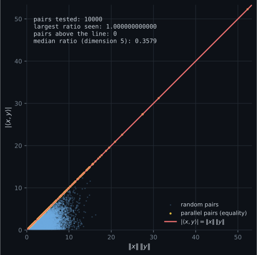
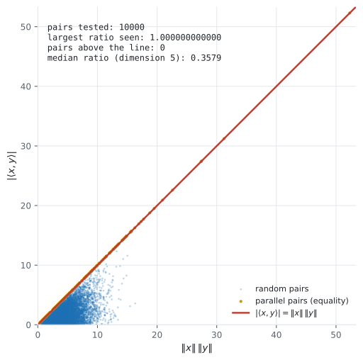
Reading the plot

From the Cauchy-Schwarz scatter. Two things. First, the bound is tight: the amber points are not merely close to the line, they are on it, with a measured ratio of $1.000000000000000$. The “if and only if” in the statement is real, and the equality case is not a measure-zero curiosity you can ignore — it is exactly the parallel pairs, which in practice means duplicated features and collinear columns.

Second, the empty region. Almost all the mass of the scatter sits well below the diagonal, and in five dimensions the median ratio over all ten thousand pairs is $0.3579$, and $0.3491$ once the planted parallel pairs are excluded. Push the dimension up and that number falls further. Two random directions in high dimensions are nearly orthogonal, which is why cosine similarity between unrelated embeddings is small rather than random-looking.

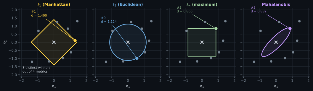
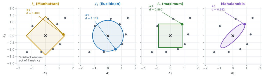
From the four metric panels. The measured winners are:

metric	nearest candidate	its distance
$\ell_1$	#1 at $(1.30, 0.10)$	$1.4000$
$\ell_2$	#9 at $(0.55, -0.98)$	$1.1238$
$\ell_\infty$	#3 at $(0.86, 0.84)$	$0.8600$
Mahalanobis	#3 at $(0.86, 0.84)$	$0.8822$

Three distinct answers from four metrics, on nine candidates. But the more striking measurement is not the winner, it is the reshuffling of the whole ranking. Under $\ell_2$ the order is #9, #4, #3, #6, #5, #2, #1, #8, #7. Under Mahalanobis it is #3, #8, #7, #6, #2, #1, #9, #4, #5. Look at two entries in particular:

• Candidate #4 at $(-0.95, 0.70)$ is the second nearest under $\ell_2$ (distance $1.180$) and the last under Mahalanobis (distance $3.121$). It runs against the correlation of the surrounding cloud, so it is an unusual point even though it is not a distant one.
• Candidate #8 at $(-1.35, -1.20)$ is eighth of nine under $\ell_2$ and second under Mahalanobis. It is further away in plain kilometres and much more typical of the data.

If your pipeline does nearest-neighbour retrieval, the choice of metric is not a tuning detail — it is the model. The $\ell_\infty$ and Mahalanobis panels happen to agree on the winner here, and they agree by coincidence: $\ell_\infty$ likes #3 because neither of its coordinates is large, and Mahalanobis likes it because it lies along the cloud’s principal direction.

Pitfalls

Ranking by dot product is not ranking by distance

Expanding $\lVert\mathbf{x}-\mathbf{y}\rVert^2 = \lVert\mathbf{x}\rVert^2 - 2\langle\mathbf{x},\mathbf{y}\rangle + \lVert\mathbf{y}\rVert^2$ shows the two agree only when every candidate has the same length. Maximum-inner-product search and nearest-neighbour search are genuinely different problems with different answers and different index structures. If you normalise your vectors first, they coincide — and that normalisation is the whole content of using cosine similarity.

Not every norm comes from an inner product

$\ell_1$ and $\ell_\infty$ are norms and induce metrics, but there is no inner product behind them. Consequently there is no angle, no orthogonality and no projection in $\ell_1$ geometry — which is why Lasso has no closed-form solution while ridge does. The parallelogram law $\lVert\mathbf{x}+\mathbf{y}\rVert^2 + \lVert\mathbf{x}-\mathbf{y}\rVert^2 = 2\lVert\mathbf{x}\rVert^2 + 2\lVert\mathbf{y}\rVert^2$ is the test: a norm comes from an inner product exactly when it satisfies that identity.

Squared distance is cheaper and is not a metric

$d^2$ fails the triangle inequality — take three collinear points at $0$, $1$, $2$: the squared distances are $1$, $1$ and $4$, and $4 > 1 + 1$. It is fine to rank by squared distance, since the square root is monotone, and it is not fine to feed squared distances to anything that assumes a metric, including most metric-tree index structures and many clustering guarantees.

Mahalanobis distance needs an invertible covariance

$\sqrt{(\mathbf{x}-\mathbf{y})^\top\Sigma^{-1}(\mathbf{x}-\mathbf{y})}$ requires $\Sigma$ to be invertible, and a covariance estimated from $n$ samples in $d$ dimensions has rank at most $\min(n-1, d)$. With $d \geq n$ it is singular. Regularise it — $\Sigma + \varepsilon\mathbf{I}$ — and report the $\varepsilon$ you used, because the resulting distances depend on it.

The zero vector has zero length, and that is a division waiting to happen

Any code that normalises by $\lVert\mathbf{x}\rVert$ — cosine similarity, unit-vector projection, Gram-Schmidt — divides by zero on the zero vector. Positive definiteness guarantees that only $\mathbf{0}$ has this problem, which is precisely why the guard is a single if and not a tolerance question.

Compare

notion	needs	gives	example that is only this
metric	three axioms on pairs	distances	edit distance on strings; shortest path on a graph
norm	metric + homogeneity + a vector space	lengths, so distances by subtraction	$\ell_1$, $\ell_\infty$
inner product	norm + the parallelogram law	lengths, distances and angles	the dot product; any SPD matrix

Reading down the table, each row buys you more structure at the cost of more assumptions. Reading up, each row is a place you can retreat to when the assumptions fail — which is what happens when you move from Euclidean data to strings, graphs or distributions.

pch.quizTag Check your understanding

1. Why is the Cauchy-Schwarz inequality needed before an angle can be defined?

   A It guarantees the inner product is positive B It bounds the ratio of the inner product to the product of the norms inside [-1, 1], which is exactly the range in which arccos is defined C It proves the inner product is symmetric D It is not needed; the angle is defined independently
   pch.quizShowAnswer

   B — It bounds the ratio of the inner product to the product of the norms inside [-1, 1], which is exactly the range in which arccos is defined — The same inequality also supplies the triangle inequality for the induced norm: expanding the squared norm of a sum and replacing the cross term by the product of the norms gives the result in one step.

2. Under the dot product, x = (1,1) has length sqrt(2). Under the book's Equation 3.19 the same vector has length exactly 1. What is going on?

   A One of the two is a rounding error B The negative off-diagonal entry subtracts a penalty proportional to x1*x2, so vectors whose coordinates agree in sign are discounted — under that inner product (1,1) is a unit vector C Equation 3.19 is not a valid inner product D The vector was normalised first
   pch.quizShowAnswer

   B — The negative off-diagonal entry subtracts a penalty proportional to x1*x2, so vectors whose coordinates agree in sign are discounted — under that inner product (1,1) is a unit vector — The matrix [[1, -0.5], [-0.5, 1]] has eigenvalues 0.5 and 1.5, so it is a perfectly valid inner product. The computation is 1 - 0.5(1+1) + 1 = 1 exactly. The book's phrasing is that this inner product 'perceives' the vector as shorter.

3. Candidate #4 in the metric figure is the second nearest of nine under the Euclidean metric and the last under Mahalanobis. Why?

   A The Mahalanobis calculation is unstable B It sits against the correlation direction of the surrounding cloud, so although it is not far in plain distance it is an atypical point — and Mahalanobis measures atypicality rather than displacement C It was not standardised D Mahalanobis distance is not a metric
   pch.quizShowAnswer

   B — It sits against the correlation direction of the surrounding cloud, so although it is not far in plain distance it is an atypical point — and Mahalanobis measures atypicality rather than displacement — Mahalanobis distance is a genuine metric, induced by the inner product with matrix Sigma-inverse. Its ranking of the nine candidates is close to a reversal of the Euclidean one at the tail: candidate #8 goes the other way, from eighth under l2 to second under Mahalanobis.

4. Which statement about squared Euclidean distance is correct?

   A It is a metric, since the square of a metric is a metric B It is not a metric — three collinear points at 0, 1 and 2 give squared distances 1, 1 and 4, and 4 exceeds 1 + 1 — but ranking by it is safe because the square root is monotone C It is a metric but not a norm D It is only a metric in one dimension
   pch.quizShowAnswer

   B — It is not a metric — three collinear points at 0, 1 and 2 give squared distances 1, 1 and 4, and 4 exceeds 1 + 1 — but ranking by it is safe because the square root is monotone — This is why you may optimise squared error freely but must not hand squared distances to a metric tree or to any argument that invokes the triangle inequality.

🧪 Try It Yourself

Exercise 1 – The induced norm from an arbitrary inner product

pch.exerciseTag pch.exerciseTitle

Exercise 2 – Try to break Cauchy-Schwarz

pch.exerciseTag pch.exerciseTitle

Exercise 3 – Show that squared distance is not a metric

pch.exerciseTag pch.exerciseTitle

Exercise 4 – Reproduce the metric disagreement

pch.exerciseTag pch.exerciseTitle

Exercise 5 – The parallelogram law tells you which norms have angles

pch.exerciseTag pch.exerciseTitle

Recall card

• The induced norm is the square root of the inner product of a vector with itself, and it is well defined precisely because the inner product is positive definite.
• Distance is the length of a difference — the same one line, applied to x minus y.
• Cauchy-Schwarz bounds the absolute inner product by the product of the two lengths, with equality exactly when the vectors are parallel; it is what makes the cosine well defined and what supplies the triangle inequality.
• A metric needs only three axioms — positive definite, symmetric, triangle inequality — and needs no vector space at all.
• Inner products sit inside norms, which sit inside metrics. The parallelogram law is the test for whether a norm has an inner product behind it, and only the Euclidean norm among the standard ones passes.
• Inner products and metrics run in opposite directions: similar means a large inner product and a small distance. Ranking by dot product equals ranking by distance only when all the vectors have equal length.
• Squared distance is not a metric — three collinear points break the triangle inequality — although ranking by it is safe.
• Changing the metric changes which point is nearest: four metrics on the same nine candidates give three different winners, and Mahalanobis nearly reverses the Euclidean ranking at the tail.

Next: Angles and Orthogonality — the second thing Cauchy-Schwarz makes possible.