Model Compression (Pruning, Quantisation and Distillation)

There are three ways to make a trained model smaller, and they work on different things. Quantisation changes how each weight is stored. Pruning removes weights. Distillation trains a different, smaller model to imitate the first one.

All three are measured here against one baseline: a 431,242-parameter convnet at 0.9733 test accuracy. Two results are worth stating before the detail:

Model	Estimated size	Accuracy	Against the baseline
Teacher (baseline)	1,684.5 KB	0.9733	—
Pruned 50%	1,263.4 KB	0.9773	+0.0040
Pruned 70%	758.0 KB	0.9760	+0.0027
Pruned 90%	252.7 KB	0.8797	−0.0936
Pruned 95%	126.3 KB	0.2477	−0.7256
Student, distilled	170.7 KB	0.9523	−0.0210

Removing half the weights made the model better, and removing 95% of them made it worse than guessing two classes. The interesting part of this page is what happens between those two rows.

What you’ll learn

• Why magnitude pruning needs a fine-tuning step, measured: it recovered +0.4863 accuracy at 90% sparsity.
• Where the cliff is, and why it is a cliff rather than a slope.
• What knowledge distillation transfers, and why it was worth only +0.0017 here.
• Why the size numbers for pruning are an estimate and quantisation’s are not.

Magnitude pruning

The rule is as simple as it sounds: set the smallest weights to zero.

Prune, then repair

threshold = np.quantile(np.abs(weights), sparsity)
pruned = np.where(np.abs(weights) < threshold, 0.0, weights)

Then fine-tune, re-applying the mask after every epoch:

The line everyone forgets

for _ in range(FINETUNE_EPOCHS):
    model.fit(x_train, y_train, epochs=1, verbose=0)
    # Gradient descent has no idea those weights are supposed to be zero, and
    # will happily refill them. Without this line the accuracy looks great and
    # the sparsity is gone.
    model.set_weights([w * m if m is not None else w
                       for w, m in zip(model.get_weights(), masks)])

That masking step is not a detail. Adam updates every weight with a non-zero gradient, including the pruned ones, so after one epoch of ordinary fine-tuning the model is dense again — with a good accuracy and none of the compression you thought you had. The measured sparsities on this page (50.00%, 69.95%, 89.98%, 94.95%, 98.98%) are checked after fine-tuning for exactly that reason.

figure 431,242 parameters, three epochs of fine-tuning after each pruning step matplotlib

The gap between the two curves is the whole technique. At 70% sparsity pruning alone costs 0.0343 and fine-tuning gives back 0.0370. At 90% the raw pruned model is at 0.3933 — barely better than chance — and fine-tuning restores it to 0.8797. Past that, at 95% and 99%, there is no longer enough capacity left to recover: +0.1177 and +0.0000.

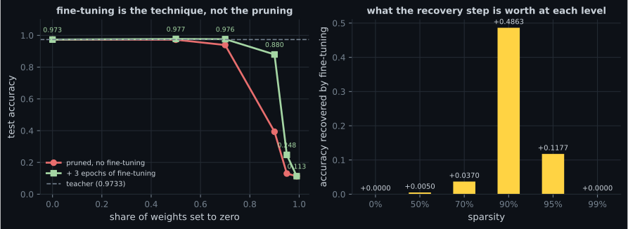
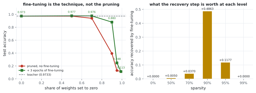
Sparsity	Pruned, no fine-tuning	Fine-tuned	Recovered
50%	0.9723	0.9773	+0.0050
70%	0.9390	0.9760	+0.0370
90%	0.3933	0.8797	+0.4863
95%	0.1300	0.2477	+0.1177
99%	0.1133	0.1133	+0.0000

Pruning half the model improved it

0.9773 against the baseline’s 0.9733. That is not a rounding artefact — it is a 0.0040 gain from deleting 215,000 weights.

The honest explanation is that removing small weights is a regulariser. A weight near zero contributes almost nothing to the forward pass but still contributes noise to the gradient of everything downstream; zeroing it and then fine-tuning lets the remaining weights re-fit without that interference. It is closely related to why dropout works, and it means “compression” and “accuracy” are not always in tension at moderate ratios.

Be careful not to over-read it: this is one run on one architecture, and a 0.0040 gain on a 3,000-sample test set is about 12 predictions. The safe claim is that pruning to 50–70% cost nothing here.

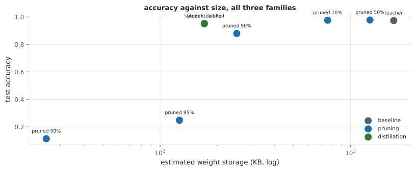
And why 95% is a cliff, not a slope

Between 90% and 95% the model goes from recoverable (0.8797) to destroyed (0.2477), and at 99% it is a constant predictor that fine-tuning cannot revive at all. Sparsity is not a dial with a smooth trade curve; there is a point where the surviving weights can no longer represent the function, and no amount of fine-tuning creates capacity that is not there.

The practical consequence: sweep it. The right sparsity for a given architecture cannot be guessed, and the difference between the last good setting and the first useless one was five percentage points here.

Distillation

A small model trained on the teacher’s soft outputs rather than on the hard labels:

$$\mathcal{L} = (1-\alpha)\,\mathcal{L}_{\text{hard}}(y, z_s) + \alpha T^2 \,\mathcal{L}_{\text{soft}}\!\left(\sigma(z_t/T),\, \sigma(z_s/T)\right)$$

The temperature $T$ flattens both distributions so the teacher’s relative opinions about wrong classes survive — that a particular 4 looks somewhat like a 9 is information the one-hot label throws away. The $T^2$ factor compensates for the gradient shrinking by $1/T^2$ when the logits are divided.

figure 43,706 parameters, 9.9x smaller than the teacher, same budget matplotlib

Distillation was worth +0.0017 here — 0.9523 against 0.9507 — which on a 3,000-sample test set is about five predictions and is not distinguishable from run-to-run noise with one seed each. The right panel shows what it is supposed to transfer: the hard label says only '4', while the teacher at T=4 also reports how much the image resembles the other classes.

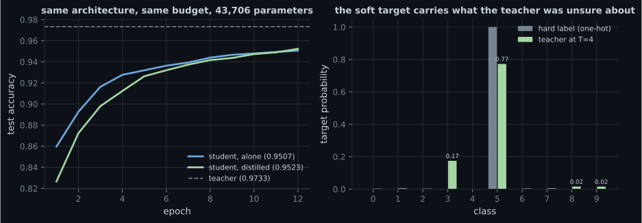
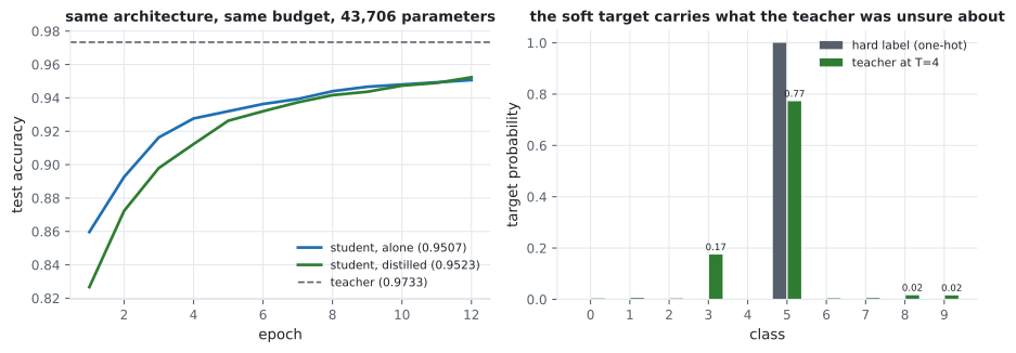
The mechanism is real and the benefit here was negligible. Both statements are supported by the figure, and the reason is that MNIST is too easy: the student alone already reaches 0.9507, so there is only 0.0226 of headroom to the teacher and very little dark knowledge to transfer. Distillation earns its reputation on harder tasks where the gap between a small model trained alone and a large one is wide.

What it did buy is the only genuinely smaller architecture on this page. Pruning leaves a 431,242-parameter model with zeros in it; the student really has 43,706 parameters, and needs no special format to benefit.

Comparing the three families

figure Every compressed model on one axis matplotlib

The two families cross. Above roughly 250 KB pruning is the better option — pruned 70% keeps 0.9760 at 758 KB. Below that it collapses, and the distilled student holds 0.9523 at 170.7 KB where pruned 90% manages only 0.8797 at 252.7 KB. Neither dominates; the crossover is what a real deployment decision turns on.

diagram Diagram mermaid

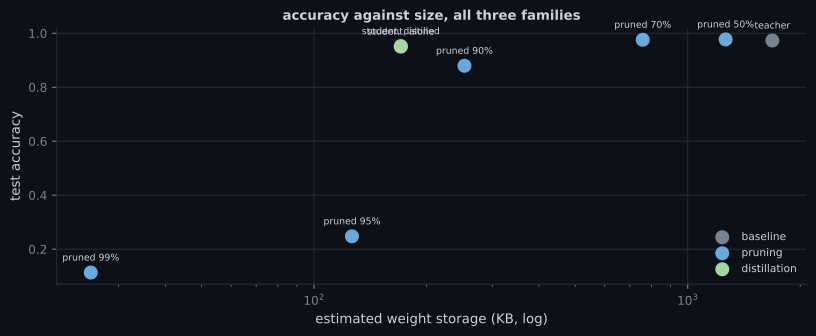
  flowchart TD
  M["trained model
431,242 params, 0.9733"] --> Q["quantisation
same weights, fewer bits"]
  M --> P["pruning
fewer weights, same shape"]
  M --> D["distillation
a different, smaller model"]
  Q -.->|"11.54x, -0.0000"| QR["see the TFLite page"]
  P -.->|"50%: +0.0040
95%: -0.7256"| PR["needs fine-tuning
and a sparse format"]
  D -.->|"9.9x smaller, -0.0210"| DR["genuinely smaller,
no special format"]

A caveat about the pruning sizes

The pruned sizes on this page are estimates, and the quantised ones on the TFLite page are measured files. The estimate assumes a sparse format costing a value plus a 16-bit index per surviving weight.

Keras writes the dense array regardless. A model pruned to 90% saved on disk is exactly the same size as the original — the zeros are stored like any other float. That saving is only real if the deployment runtime supports a sparse format, and many do not. Quantisation’s saving needs no such cooperation, which is a large practical advantage that the accuracy numbers alone do not show.

The three also compose: pruning then quantising a model applies both reductions, and the TFLite converter will happily quantise a model full of zeros.

sketch What magnitude pruning removes p5.js Pause Restart

Drag the sparsity slider. The bars are a weight distribution; the dimmed ones are set to zero, and the readout gives the measured accuracy at that level.

sketch The measured table, ranked p5.js Pause Restart

Click a column to rank every row by it. The bars are that column's values and the highest and lowest are computed from the numbers, not written in.

Pitfalls

• Fine-tuning without re-applying the mask. Gradient descent refills the pruned weights; the accuracy looks fine and the sparsity is gone.
• Reporting pruning as a size saving without a sparse format. A dense file of mostly zeros is the same size as a dense file of weights.
• Assuming sparsity trades smoothly. 90% recovered to 0.8797 and 95% to 0.2477.
• Skipping the fine-tuning step and concluding pruning does not work. At 90% that is the difference between 0.3933 and 0.8797.
• Reading +0.0040 or +0.0017 as a real improvement. On a 3,000-sample test set those are roughly 12 and 5 predictions, from one seed.
• Expecting distillation to shine on an easy task. The student alone was already within 0.0226 of the teacher.
• Forgetting the $T^2$ factor. Dividing logits by $T$ shrinks the gradient by $1/T^2$, so the soft term silently stops contributing.

Recap

• Pruning to 50% improved accuracy to 0.9773 against 0.9733, acting as a regulariser.
• Fine-tuning after pruning is the technique: worth +0.4863 at 90% sparsity.
• The failure is a cliff, not a slope — 0.8797 at 90%, 0.2477 at 95%, 0.1133 at 99%.
• Distillation gave a 9.9× smaller model at 0.9523, worth +0.0017 over training the same student alone, which is within noise here.
• Pruning’s size saving depends on a sparse deployment format; quantisation’s does not.
• Above ~250 KB pruning won, below it the distilled student won — the families cross.

Next

Compression assumes the model is finished. The other way to spend a fixed budget is on finding a better model in the first place: Hyperparameter Tuning with KerasTuner.

pch.quizTag pch.quizDefaultTitle

1. Pruning 50% of the weights raised accuracy from 0.9733 to 0.9773. How can deleting weights help?

   A The measurement must be wrong B Removing near-zero weights acts as a regulariser — they contribute almost nothing to the forward pass but add noise downstream, so the remaining weights re-fit better once they are gone C Pruning increases the learning rate D The pruned model was trained for longer
   pch.quizShowAnswer

   B — Removing near-zero weights acts as a regulariser — they contribute almost nothing to the forward pass but add noise downstream, so the remaining weights re-fit better once they are gone — It is closely related to why dropout works. The gain is small — about 12 predictions on a 3,000-sample test set — so the safe claim is that pruning to 50% cost nothing.

2. Why must the pruning mask be re-applied after every fine-tuning epoch?

   A To keep the file size down B Because gradient descent updates every weight with a non-zero gradient, including the pruned ones — after one ordinary epoch the model is dense again, with good accuracy and no compression C Because Keras resets weights between epochs D To prevent overfitting
   pch.quizShowAnswer

   B — Because gradient descent updates every weight with a non-zero gradient, including the pruned ones — after one ordinary epoch the model is dense again, with good accuracy and no compression — This is why the measured sparsities are checked after fine-tuning: 50.00%, 69.95%, 89.98%, and so on.

3. Accuracy after fine-tuning was 0.8797 at 90% sparsity and 0.2477 at 95%. What does that shape tell you?

   A The fine-tuning budget was too small at 95% B Sparsity is not a smooth trade — there is a point where the surviving weights cannot represent the function, and fine-tuning cannot create capacity that is not there C The model was badly initialised D 95% sparsity is always too aggressive
   pch.quizShowAnswer

   B — Sparsity is not a smooth trade — there is a point where the surviving weights cannot represent the function, and fine-tuning cannot create capacity that is not there — Fine-tuning recovered +0.4863 at 90% and only +0.1177 at 95%, so the recovery mechanism itself breaks down rather than merely needing more epochs.

4. Distillation produced 0.9523 against 0.9507 for the same student trained alone. What is the honest conclusion?

   A Distillation does not work B The mechanism is real but the benefit here is negligible and within noise — MNIST is easy enough that the student alone was already within 0.0226 of the teacher, leaving little to transfer C The temperature was set wrongly D The student was too large
   pch.quizShowAnswer

   B — The mechanism is real but the benefit here is negligible and within noise — MNIST is easy enough that the student alone was already within 0.0226 of the teacher, leaving little to transfer — Distillation earns its reputation where the gap between a small model trained alone and a large one is wide, which is not the case here.

5. Why are the pruned model sizes on this page called estimates while the quantised sizes on the TFLite page are not?

   A Pruning is less precise than quantisation B Keras stores zeros like any other float, so a pruned model on disk is the same size as the original — the saving only exists if the deployment runtime supports a sparse format, whereas quantisation needs no such cooperation C The estimate ignores the biases D Pruned models cannot be saved
   pch.quizShowAnswer

   B — Keras stores zeros like any other float, so a pruned model on disk is the same size as the original — the saving only exists if the deployment runtime supports a sparse format, whereas quantisation needs no such cooperation — The estimate assumes a value plus a 16-bit index per surviving weight, which is what a CSR-style format costs — but nothing in the standard save path produces that.

🧪 Try It Yourself

pch.exerciseTag pch.exerciseTitle

pch.exerciseTag pch.exerciseTitle

pch.exerciseTag pch.exerciseTitle

pch.exerciseTag pch.exerciseTitle

pch.exerciseTag pch.exerciseTitle

pch.exerciseTag pch.exerciseTitle