Why the Margin Can Be Set to One

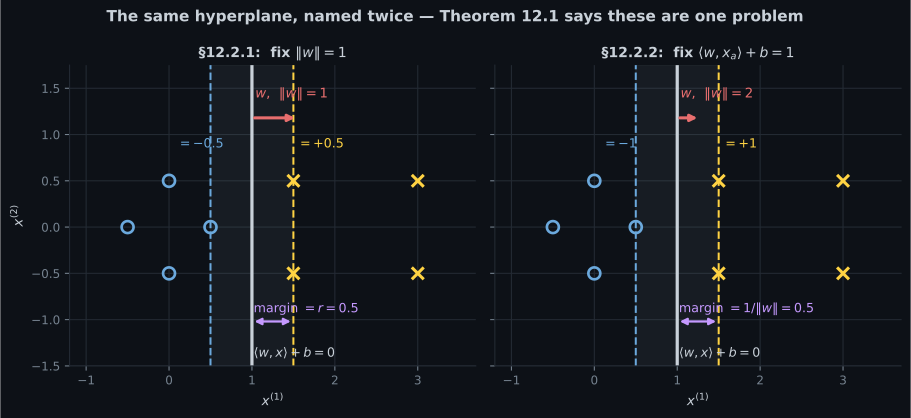
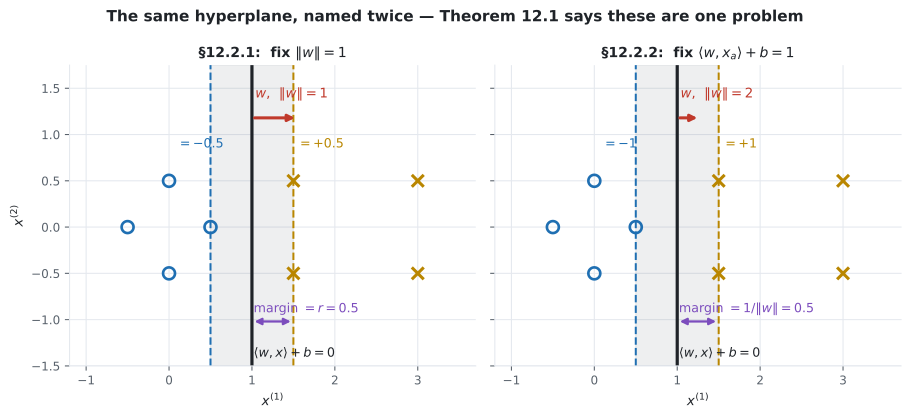
Page 1202 spent the scale freedom one way: demand $\lVert\mathbf{w}\rVert = 1$, and read the margin off as a separate variable $r$. Section 12.2.2 spends it the other way — demand that the predictor’s value at the closest example be exactly $1$ — and Section 12.2.3 proves the two give the same classifier.

The derivation

Let $\mathbf{x}_a$ be the closest example, scaled so that $\langle\mathbf{w},\mathbf{x}_a\rangle + b = 1$. Its projection $\mathbf{x}_a'$ is on the hyperplane:

$$\langle\mathbf{w}, \mathbf{x}_a'\rangle + b = 0 \qquad \text{(12.11)}$$

Substitute Equation 12.8, $\mathbf{x}_a' = \mathbf{x}_a - r\,\mathbf{w}/\lVert\mathbf{w}\rVert$:

$$\Big\langle \mathbf{w},\ \mathbf{x}_a - r\frac{\mathbf{w}}{\lVert\mathbf{w}\rVert}\Big\rangle + b = 0 \qquad \text{(12.12)}$$

and expand by bilinearity:

$$\underbrace{\langle\mathbf{w},\mathbf{x}_a\rangle + b}_{=\ 1} \ -\ r\,\frac{\overbrace{\langle\mathbf{w},\mathbf{w}\rangle}^{=\ \lVert\mathbf{w}\rVert^2}}{\lVert\mathbf{w}\rVert} = 0 \qquad \text{(12.13)}$$

The second fraction is $r\lVert\mathbf{w}\rVert$, so $1 - r\lVert\mathbf{w}\rVert = 0$ and

$$r = \frac{1}{\lVert\mathbf{w}\rVert} \qquad \text{(12.14)}$$

Two lines, and the margin is now a function of the parameters rather than a variable of its own. That is the entire content of §12.2.2 — the rest is bookkeeping.

the_derivation.py

import numpy as np
 
X = np.array([[3.0,  1.0], [3.0, -1.0], [6.0,  1.0], [6.0, -1.0],
              [1.0,  0.0], [0.0,  1.0], [0.0, -1.0], [-1.0, 0.0]])
Y = np.array([ 1.0,  1.0,  1.0,  1.0,  -1.0, -1.0, -1.0, -1.0])
w, b = np.array([1.0, 0.0]), -2.0
 
xa = X[0]                                       # (3, 1), a closest positive
nw = np.linalg.norm(w)
r  = (w @ xa + b) / nw
xp = xa - r * w / nw
 
print(f"<w, x_a> + b                  : {w @ xa + b:.10f}")
print(f"12.11: <w, x'_a> + b          : {w @ xp + b:.3e}")
print(f"12.13: LHS                    : "
      f"{w @ xa + b - r * (w @ w) / nw:.3e}")
print(f"12.14: 1/||w||                : {1/nw:.10f}")
print(f"       measured distance      : {np.linalg.norm(xa - xp):.10f}")

text

<w, x_a> + b                  : 1.0000000000
12.11: <w, x'_a> + b          : 0.000e+00
12.13: LHS                    : 0.000e+00
12.14: 1/||w||                : 1.0000000000
       measured distance      : 1.0000000000

Equation 12.14 is not special to this example. Over $20{,}000$ random $(\mathbf{w}, b)$ and random points, with the scale condition imposed, the worst disagreement between the measured distance and $1/\lVert\mathbf{w}\rVert$ is $3.553\times10^{-15}$.

figure The same hyperplane, named twice — Theorem 12.1 says these are one problem matplotlib

Drawn on the running example halved, so the margin is 0.5 rather than 1 and the two parametrisations are visibly different. Left, the margin is the variable r. Right, the level sets are pinned at ±1 and the margin is 1/||w||. The black line, the shaded band and the classifier are the same object in both.

The hard margin SVM

With the margin now equal to $1/\lVert\mathbf{w}\rVert$, the requirement that every point be at least a margin away becomes

$$y_n(\langle\mathbf{w},\mathbf{x}_n\rangle + b) \geq 1 \qquad \text{(12.15)}$$

and the objective is to make $1/\lVert\mathbf{w}\rVert$ as large as possible:

$$\max_{\mathbf{w},b}\ \frac{1}{\lVert\mathbf{w}\rVert} \quad\text{subject to}\quad y_n(\langle\mathbf{w},\mathbf{x}_n\rangle + b) \geq 1 \ \text{ for all } n \qquad \text{(12.16), (12.17)}$$

The book then says: “Instead of maximizing the reciprocal of the norm as in (12.16), we often minimize the squared norm. We also often include a constant $\tfrac12$ that does not affect the optimal $\mathbf{w}, b$ but yields a tidier form when we compute the gradient.”

$$\min_{\mathbf{w},b}\ \tfrac12\lVert\mathbf{w}\rVert^2 \quad\text{subject to}\quad y_n(\langle\mathbf{w},\mathbf{x}_n\rangle + b) \geq 1 \ \text{ for all } n \qquad \text{(12.18), (12.19)}$$

This is the hard margin SVM — “hard” because the constraints admit no violations at all.

does_squaring_change_it.py

from scipy.optimize import minimize
 
def solve(obj, seed=0):
    rg = np.random.default_rng(seed)
    return minimize(obj, np.r_[rg.normal(0, 1, 2), rg.normal(0, 1)],
                    constraints=[{"type": "ineq",
                                  "fun": lambda v: Y * (X @ v[:2] + v[2]) - 1}],
                    method="SLSQP", options={"maxiter": 6000, "ftol": 1e-14})
 
r1 = solve(lambda v: np.linalg.norm(v[:2]))     # 12.16, as written
r2 = solve(lambda v: 0.5 * v[:2] @ v[:2])       # 12.18, squared
print(f"minimising ||w||      : w = {np.round(r1.x[:2], 8)}, b = {r1.x[2]:.8f}")
print(f"minimising 0.5||w||^2 : w = {np.round(r2.x[:2], 8)}, b = {r2.x[2]:.8f}")
print(f"largest difference    : {np.abs(r1.x - r2.x).max():.3e}")

text

minimising ||w||      : w = [1. 0.], b = -2.00000000
minimising 0.5||w||^2 : w = [1. 0.], b = -2.00000000
largest difference    : 4.441e-16

The objective values differ — $1.0$ against $0.5$ — and the argmin does not, because $t \mapsto \tfrac12 t^2$ is strictly increasing on $t \geq 0$. That is the whole justification, and it is worth noticing that it depends on $\lVert\mathbf{w}\rVert$ being non-negative; the same move on a quantity that could be negative would be wrong.

What squaring actually buys, measured

The book’s reason is cosmetic — “a tidier form when we compute the gradient”. The real payoff is structural: $\lVert\mathbf{w}\rVert$ is not differentiable at $\mathbf{w} = \mathbf{0}$, while $\tfrac12\lVert\mathbf{w}\rVert^2$ is smooth everywhere with constant Hessian $\mathbf{I}$. That makes 12.18 a convex quadratic program, the object §12.5 hands to a standard solver.

Over $500$ random starting points on the running example:

objective	failures	median iterations	worst iterations
$\lVert\mathbf{w}\rVert$	$3$ of $500$	$3$	$\mathbf{29}$
$\tfrac12\lVert\mathbf{w}\rVert^2$	$\mathbf{0}$ of $500$	$2$	$\mathbf{5}$

Started exactly at $\mathbf{w} = \mathbf{0}$ — the point where the norm is not differentiable — both still converge in two iterations, because the constraints immediately push the iterate away from the origin. The difference does not show up in a single unlucky start; it shows up across many.

Theorem 12.1, and what its proof turns on

Theorem 12.1. Maximizing the margin $r$, where we consider normalized weights as in (12.10), is equivalent to scaling the data, such that the margin is unity.

The proof is four steps, and only one of them is doing work:

1. Square the objective. Maximising $r$ and maximising $r^2$ have the same argmax for $r \geq 0$.
2. Reparametrise. Replace the normalised $\mathbf{w}$ by $\mathbf{w}'/\lVert\mathbf{w}'\rVert$ for an unconstrained $\mathbf{w}'$, giving Equation 12.22.
3. Divide the constraint by $r$. Legitimate because $r > 0$ — which is where linear separability is used. Define $\mathbf{w}'' = \mathbf{w}'/(\lVert\mathbf{w}'\rVert r)$ and $b'' = b/r$, Equation 12.23.
4. Read off the norm. $\lVert\mathbf{w}''\rVert = 1/r$, Equation 12.24, so maximising $r^2$ is maximising $1/\lVert\mathbf{w}''\rVert^2$, which is minimising $\tfrac12\lVert\mathbf{w}''\rVert^2$.

Step 4 is the hinge. Checked over $50{,}000$ random $(\mathbf{w}', r)$ draws, the worst deviation of $\lVert\mathbf{w}''\rVert$ from $1/r$ is $1.137\times10^{-13}$.

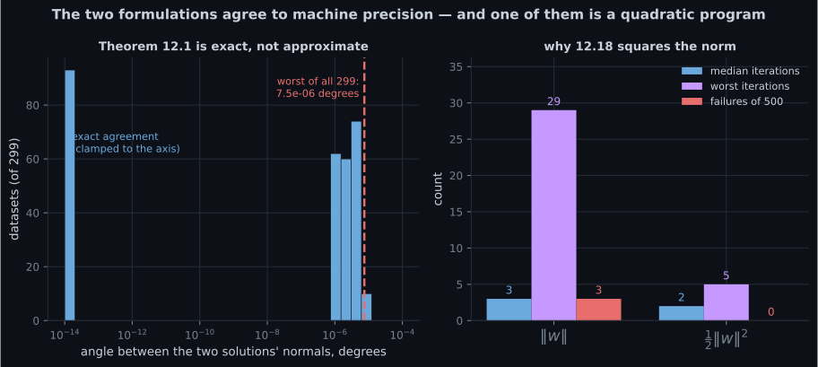
And the theorem itself, on $300$ random datasets of dimension $2$ to $5$ and size $6$ to $15$:

theorem_12_1.py

# solve both formulations on the same data, then compare the HYPERPLANES
rg = np.random.default_rng(3)
angs, rgaps = [], []
while len(angs) < 299:
    D, n = int(rg.integers(2, 6)), int(rg.integers(6, 16))
    mu = rg.normal(0, 1, D) * 3
    XX = np.vstack([rg.normal(mu, 1.0, (n // 2, D)),
                    rg.normal(-mu, 1.0, (n - n // 2, D))])
    YY = np.r_[np.ones(n // 2), -np.ones(n - n // 2)]
    a = best_1221(XX, YY)            # min 0.5||w||^2
    c = best_1210(XX, YY)            # max r, ||w|| = 1
    if a is None or c is None:
        continue
    wa = a.x[:D] / np.linalg.norm(a.x[:D])
    wc = c.x[:D] / np.linalg.norm(c.x[:D])
    wc = wc if wa @ wc >= 0 else -wc
    angs.append(np.degrees(np.arccos(np.clip(wa @ wc, -1, 1))))
    rgaps.append(abs(c.x[D + 1] - 1.0 / np.linalg.norm(a.x[:D])))
 
print(f"worst angle between normals     : {max(angs):.3e} degrees")
print(f"worst |r - 1/||w|||             : {max(rgaps):.3e}")

text

worst angle between normals     : 7.492e-06 degrees
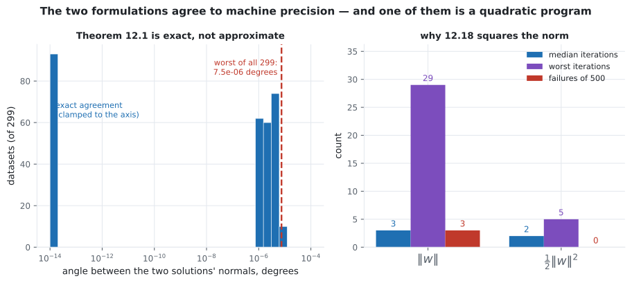
worst |r - 1/||w|||             : 2.327e-13

Seven millionths of a degree, across three hundred problems. The two formulations do not approximately agree — they return the same hyperplane, and the residual is solver tolerance rather than any difference in the mathematics.

figure The two formulations agree to machine precision — and one of them is a quadratic program matplotlib

Left: a third of the datasets agree exactly, and the rest sit at solver tolerance. Right: what Section 12.2.2's squared norm is really for. It is not about a tidier gradient — it is about handing Section 12.5 a convex quadratic program.

One dataset out of 300 did not finish

Of the $300$ datasets, $\mathbf{299}$ produced a comparison. On one of them the $\lVert\mathbf{w}\rVert = 1$ formulation failed to converge from any of its ten starting points, while the squared-norm formulation converged from the first.

That is page 1202’s non-convexity showing up again at a rate of about one problem in three hundred. Theorem 12.1 says the two problems have the same solution; it does not say they are equally easy to solve, and in practice nobody solves Equation 12.10.

pch.quizTag Check your understanding

1. A From the constraint y_n f(x_n) >= 1 B From the scale choice of Section 12.2.2: x_a is the closest example and the data has been scaled so that its predictor value is exactly 1 C From the norm of w being 1 D From the label y_a being +1
   pch.quizShowAnswer

   B — From the scale choice of Section 12.2.2: x_a is the closest example and the data has been scaled so that its predictor value is exactly 1

2. A They have the same objective value B Because ||w|| is always 1 C Because t maps to half t squared is strictly increasing on non-negative t, so the argmin is unchanged — measured, the two solutions differ by 4.441e-16 while the objective values differ by a factor of two D Because the constraint set is convex
   pch.quizShowAnswer

   C — Because t maps to half t squared is strictly increasing on non-negative t, so the argmin is unchanged — measured, the two solutions differ by 4.441e-16 while the objective values differ by a factor of two

3. A It makes the objective smaller B The norm is not differentiable at the origin, whereas the squared norm is smooth with constant Hessian — making 12.18 a convex quadratic program. Over 500 starts, the norm form failed 3 times and needed up to 29 iterations; the squared form failed 0 times and needed at most 5 C It removes the need for constraints D It makes the problem non-convex
   pch.quizShowAnswer

   B — The norm is not differentiable at the origin, whereas the squared norm is smooth with constant Hessian — making 12.18 a convex quadratic program. Over 500 starts, the norm form failed 3 times and needed up to 29 iterations; the squared form failed 0 times and needed at most 5

4. A The dataset was not linearly separable B The two formulations genuinely disagreed there C The ||w|| = 1 formulation failed to converge from all ten of its starting points, while the squared-norm one converged from the first — the non-convex sphere constraint again D The dimension was too high
   pch.quizShowAnswer

   C — The ||w|| = 1 formulation failed to converge from all ten of its starting points, while the squared-norm one converged from the first — the non-convex sphere constraint again

Exercises

Exercise 1 – Derive r = 1/||w|| numerically

pch.exerciseTag pch.exerciseTitle

Exercise 2 – Check step 12.24 of the proof

pch.exerciseTag pch.exerciseTitle

Exercise 3 – Count the iterations each objective needs

pch.exerciseTag pch.exerciseTitle

Recall card

• Section 12.2.2 spends the scale freedom the other way: instead of demanding a unit-length w, it demands that the predictor’s value at the closest example be exactly one.
• Two lines of algebra then give r equal to one over the norm of w — substitute the projection into the hyperplane equation and use bilinearity. Verified to 3.553e-15 over twenty thousand random draws.
• The margin stops being a variable and becomes a function of the parameters, which is what makes the rest of the chapter possible.
• The hard margin SVM minimises half the squared norm subject to every point having margin at least one. Hard means no violations are allowed at all.
• Squaring the norm does not move the answer, only the objective value — measured, the two solutions differ by 4.441e-16 while the values differ by a factor of two.
• But squaring buys something real. The norm is not differentiable at the origin and the squared norm is smooth with constant Hessian, so 12.18 is a convex quadratic program.
• Measured over five hundred starts: the norm objective failed three times and took up to twenty-nine iterations; the squared objective never failed and never took more than five.
• Theorem 12.1 says the two formulations are equivalent, and its proof turns on one step — the reparametrised weight vector has norm exactly one over r, checked to 1.137e-13.
• That step needs r greater than zero, which is where linear separability enters the proof and nowhere else.
• Measured on three hundred random datasets, the two formulations agree to 7.492e-06 degrees. They do not approximately agree; the residual is solver tolerance.
• On one dataset in three hundred the normalised formulation did not converge at all, while the convex one did. Equivalent problems are not equally easy problems, and nobody solves Equation 12.10 in practice.

Next: The Soft Margin SVM — §12.2.4, what to do when no separating hyperplane exists at all.