Singular Value Decomposition

Everything so far has had a hypothesis. Cholesky needs symmetric positive definite. The eigendecomposition needs square and non-defective. Both hypotheses fail on ordinary data — a $1000 \times 30$ table of measurements is not square, so neither applies.

The singular value decomposition has no hypothesis. It exists for every real matrix of every shape, which is why Strang called it the fundamental theorem of linear algebra. And it does more than merely exist: it hands you the rank, the four fundamental subspaces, the pseudo-inverse, and — next page — the provably best low-rank approximation.

What you’ll learn

• Theorem 4.22: the statement of the SVD, and why $\boldsymbol{\Sigma}$ is rectangular with zero padding.
• The geometry: $\mathbf{V}^\top$ rotates in the domain, $\boldsymbol{\Sigma}$ scales and changes dimension, $\mathbf{U}$ rotates in the codomain.
• Why $\mathbf{U}$ and $\mathbf{V}$ are not inverses of each other, unlike $\mathbf{P}$ and $\mathbf{P}^{-1}$.
• §4.5.2’s construction: $\mathbf{V}$ from $\mathbf{A}^\top\mathbf{A}$, $\mathbf{U}$ from $\mathbf{A}\mathbf{A}^\top$, joined by $\mathbf{u}_i = \mathbf{A}\mathbf{v}_i/\sigma_i$.
• The singular value equation $\mathbf{A}\mathbf{v}_i = \sigma_i\mathbf{u}_i$, and how it differs from the eigenvalue equation.
• §4.5.3: every difference between the eigendecomposition and the SVD, measured rather than asserted.
• The full, reduced and truncated conventions, so you can read any paper’s notation.

Intuition: two rooms and a doorway

The eigendecomposition works inside one room. It changes into a better basis, scales, and changes back — and because it starts and ends in the same room, the two basis changes are inverse to each other.

The SVD connects two rooms of possibly different size. $\mathbf{V}^\top$ finds the best axes in the domain. $\boldsymbol{\Sigma}$ carries you through the doorway, stretching along those axes and either padding with zeros (if the codomain is bigger) or dropping coordinates (if it is smaller). $\mathbf{U}$ then finds the best axes in the codomain. Both basis changes are rotations, but they rotate in different spaces, so they cannot be inverses of each other. What links them is $\boldsymbol{\Sigma}$.

diagram Diagram mermaid

  flowchart LR
  X["x in R^n
standard basis"] -->|"Vᵀ
rotate in the domain"| XB["coordinates in
the v-basis"]
  XB -->|"Σ
scale by σᵢ,
pad or drop dimensions"| YB["coordinates in
the u-basis, in R^m"]
  YB -->|"U
rotate in the codomain"| Y["Ax in R^m
standard basis"]
  X -->|"A, directly"| Y

diagram Diagram mermaid

  flowchart TD
  EVD["eigendecomposition
A = P D P⁻¹"]
  SVD["SVD
A = U Σ Vᵀ"]
  EVD --> E1["needs square"]
  EVD --> E2["needs non-defective"]
  EVD --> E3["P and P⁻¹ are inverses:
ONE room"]
  EVD --> E4["D may be negative
or complex"]
  SVD --> S1["any shape"]
  SVD --> S2["always exists"]
  SVD --> S3["U and V are DIFFERENT
rotations in TWO rooms"]
  SVD --> S4["Σ is real and
non-negative"]
  E3 --> SAME["for a symmetric matrix
the two coincide
— spectral theorem"]
  S3 --> SAME

The math

Theorem 4.22 — SVD Theorem

Let $\mathbf{A} \in \mathbb{R}^{m\times n}$ be a rectangular matrix of rank $r \in [0, \min(m,n)]$. The SVD of $\mathbf{A}$ is a decomposition of the form

$$\mathbf{A} = \mathbf{U}\,\boldsymbol{\Sigma}\,\mathbf{V}^\top \tag{4.64}$$

with an orthogonal matrix $\mathbf{U} \in \mathbb{R}^{m\times m}$ with column vectors $\mathbf{u}_i$, $i = 1,\dots,m$, and an orthogonal matrix $\mathbf{V} \in \mathbb{R}^{n\times n}$ with column vectors $\mathbf{v}_j$, $j = 1,\dots,n$. Moreover, $\boldsymbol{\Sigma}$ is an $m\times n$ matrix with $\Sigma_{ii} = \sigma_i \geq 0$ and $\Sigma_{ij} = 0$ for $i \neq j$.

The diagonal entries $\sigma_i$, $i = 1,\dots,r$, are the singular values, the $\mathbf{u}_i$ are the left-singular vectors, and the $\mathbf{v}_j$ the right-singular vectors. By convention they are ordered: $\sigma_1 \geq \sigma_2 \geq \dots \geq \sigma_r \geq 0$.

Three things in that statement deserve emphasis.

$\boldsymbol{\Sigma}$ is the same shape as $\mathbf{A}$. Not square. The singular value matrix is unique, and it needs zero padding to fit. If $m > n$ it is diagonal down to row $n$ and then all-zero rows (Equation 4.65); if $m < n$ it is diagonal across to column $m$ and then all-zero columns (Equation 4.66):

$$m > n:\quad \boldsymbol{\Sigma} = \begin{bmatrix}\sigma_1 & 0 & 0\\ 0 & \ddots & 0\\ 0 & 0 & \sigma_n\\ 0 & \cdots & 0\\ \vdots & & \vdots\\ 0 & \cdots & 0\end{bmatrix} \qquad m < n:\quad \boldsymbol{\Sigma} = \begin{bmatrix}\sigma_1 & 0 & 0 & 0 & \cdots & 0\\ 0 & \ddots & 0 & 0 & & 0\\ 0 & 0 & \sigma_m & 0 & \cdots & 0\end{bmatrix}$$

Both outer matrices are orthogonal. So both are rigid motions — rotations, possibly with a reflection. Nothing in the SVD shears. All the stretching lives in the middle, in real non-negative numbers.

$r$ can be $0$. Rank zero means the zero matrix, and its SVD is $\boldsymbol{\Sigma} = \mathbf{0}$ with any orthogonal $\mathbf{U}$, $\mathbf{V}$. The theorem genuinely covers everything.

The geometry, in three steps

Assume $\Phi: \mathbb{R}^n \to \mathbb{R}^m$ with standard bases $B$ and $C$, and a second basis $\tilde{B}$ of $\mathbb{R}^n$ and $\tilde{C}$ of $\mathbb{R}^m$. Then, following the book:

step	what it does
$\mathbf{V}^\top = \mathbf{V}^{-1}$	a basis change in the domain $\mathbb{R}^n$, from $B$ into $\tilde{B}$ — the right-singular vectors become aligned with the coordinate axes
$\boldsymbol{\Sigma}$	scales the new coordinates by the $\sigma_i$ and adds or deletes dimensions; it is the matrix of $\Phi$ with respect to $\tilde{B}$ and $\tilde{C}$
$\mathbf{U}$	a basis change in the codomain $\mathbb{R}^m$, from $\tilde{C}$ into the canonical basis of $\mathbb{R}^m$

The book’s own summary is the sentence to keep: the SVD expresses a change of basis in both the domain and the codomain, in contrast with the eigendecomposition, which operates within the same vector space, applying one basis change and then undoing it. What makes the SVD special is that the two different bases are simultaneously linked by $\boldsymbol{\Sigma}$.

Constructing it (§4.5.2)

The derivation is short and it is the reason the spectral theorem was worth remembering.

Step 1 — $\mathbf{V}$ from $\mathbf{A}^\top\mathbf{A}$. Substitute the SVD into $\mathbf{A}^\top\mathbf{A}$, which is symmetric whatever $\mathbf{A}$ is:

$$\mathbf{A}^\top\mathbf{A} = (\mathbf{U}\boldsymbol{\Sigma}\mathbf{V}^\top)^\top(\mathbf{U}\boldsymbol{\Sigma}\mathbf{V}^\top) = \mathbf{V}\boldsymbol{\Sigma}^\top\mathbf{U}^\top\mathbf{U}\boldsymbol{\Sigma}\mathbf{V}^\top = \mathbf{V}\begin{bmatrix}\sigma_1^2 & & 0\\ & \ddots & \\ 0 & & \sigma_n^2\end{bmatrix}\mathbf{V}^\top \tag{4.73}$$

using $\mathbf{U}^\top\mathbf{U} = \mathbf{I}$. Compare with the eigendecomposition $\mathbf{A}^\top\mathbf{A} = \mathbf{P}\mathbf{D}\mathbf{P}^{-1}$: the spectral theorem guarantees one exists with an orthonormal $\mathbf{P}$, so the eigenvectors of $\mathbf{A}^\top\mathbf{A}$ are the right-singular vectors $\mathbf{V}$, and its eigenvalues are the squared singular values.

Step 2 — $\mathbf{U}$ from $\mathbf{A}\mathbf{A}^\top$. The same substitution the other way round (Equation 4.76) gives $\mathbf{A}\mathbf{A}^\top = \mathbf{U}\,\mathrm{diag}(\sigma_1^2,\dots,\sigma_m^2)\,\mathbf{U}^\top$, so the orthonormal eigenvectors of $\mathbf{A}\mathbf{A}^\top$ are the left-singular vectors. And since $\mathbf{A}\mathbf{A}^\top$ and $\mathbf{A}^\top\mathbf{A}$ have the same nonzero eigenvalues, the nonzero entries of $\boldsymbol{\Sigma}$ come out the same either way.

Step 3 — join them. The images of the $\mathbf{v}_i$ under $\mathbf{A}$ are already orthogonal:

$$(\mathbf{A}\mathbf{v}_i)^\top(\mathbf{A}\mathbf{v}_j) = \mathbf{v}_i^\top(\mathbf{A}^\top\mathbf{A})\mathbf{v}_j = \mathbf{v}_i^\top(\lambda_j\mathbf{v}_j) = \lambda_j\,\mathbf{v}_i^\top\mathbf{v}_j = 0 \tag{4.77}$$

for $i \neq j$. So normalise them:

$$\mathbf{u}_i := \frac{\mathbf{A}\mathbf{v}_i}{\lVert\mathbf{A}\mathbf{v}_i\rVert} = \frac{1}{\sqrt{\lambda_i}}\mathbf{A}\mathbf{v}_i = \frac{1}{\sigma_i}\mathbf{A}\mathbf{v}_i \tag{4.78}$$

Rearranged, that is the singular value equation:

$$\mathbf{A}\mathbf{v}_i = \sigma_i\mathbf{u}_i, \qquad i = 1,\dots,r \tag{4.79}$$

which closely resembles the eigenvalue equation $\mathbf{A}\mathbf{x} = \lambda\mathbf{x}$ — except that the vectors on the two sides are not the same vector. Collecting columns gives $\mathbf{A}\mathbf{V} = \mathbf{U}\boldsymbol{\Sigma}$ (Equation 4.80), and right-multiplying by $\mathbf{V}^\top$ gives Theorem 4.22.

A free basis for the kernel

For $m > n$, Equation 4.79 holds only for $i \leq n$; for $n > m$ it holds only for $i \leq m$, and for $i > m$ we have $\mathbf{A}\mathbf{v}_i = \mathbf{0}$ while the $\mathbf{v}_i$ are still orthonormal. So the SVD also supplies an orthonormal basis of the kernel of $\mathbf{A}$ — the trailing columns of $\mathbf{V}$. You get the null space for free, which is what §2.7.3 had to work for.

The eigendecomposition against the SVD (§4.5.3)

	eigendecomposition $\mathbf{P}\mathbf{D}\mathbf{P}^{-1}$	SVD $\mathbf{U}\boldsymbol{\Sigma}\mathbf{V}^\top$
exists for	square, and only if a basis of eigenvectors exists	every $\mathbb{R}^{m\times n}$
domain and codomain	the same space	possibly different dimensions
are the outer matrices orthonormal?	$\mathbf{P}$’s columns are not necessarily	$\mathbf{U}$ and $\mathbf{V}$ always are
are they inverse to each other?	yes	no — they change basis in different spaces
middle factor	may be negative or complex	all real and non-negative
left factor’s columns are eigenvectors of	$\mathbf{A}$	$\mathbf{A}\mathbf{A}^\top$
right factor’s columns are eigenvectors of	—	$\mathbf{A}^\top\mathbf{A}$
for a symmetric matrix	the two are one and the same, by the spectral theorem

That last row is the bridge. Symmetry collapses the two decompositions into each other — which is why Chapter 10 can describe PCA either way and get the same answer.

Three conventions you will meet

The mathematics is invariant to these; the notation is not.

name	shapes, for $m \geq n$	why anyone uses it
full SVD — Equation 4.64, used here	$\mathbf{U}$ is $m\times m$, $\boldsymbol{\Sigma}$ is $m\times n$, $\mathbf{V}$ is $n\times n$	both outer matrices are square and orthogonal; you get bases for all four subspaces
reduced SVD — Equation 4.89	$\mathbf{U}$ is $m\times n$, $\boldsymbol{\Sigma}$ is $n\times n$, $\mathbf{V}$ is $n\times n$	$\boldsymbol{\Sigma}$ is square and diagonal, as in the eigendecomposition
truncated SVD — §4.6	$\mathbf{U}$ is $m\times r$, $\boldsymbol{\Sigma}$ is $r\times r$, $\mathbf{V}$ is $r\times n$	$\boldsymbol{\Sigma}$ has no zeros on its diagonal at all; this is the approximation of the next page

In NumPy, full_matrices=True (the default) gives the full SVD and full_matrices=False gives the reduced one. The book notes that a restriction to $m > n$ is practically unnecessary: when $m < n$, $\boldsymbol{\Sigma}$ simply has more zero columns than rows and $\sigma_{m+1},\dots,\sigma_n$ are zero.

From the book

Section 4.5. Theorem 4.22 (Equation 4.64) states the SVD, with Equations 4.65 and 4.66 giving the zero padding of $\boldsymbol{\Sigma}$ for $m > n$ and $m < n$. Section 4.5.1 gives the geometric intuition as three steps — Figure 4.8 draws it for a $3\times2$ matrix and Figure 4.9 applies it to a grid of vectors, worked as Example 4.12 (Equation 4.67). Section 4.5.2 constructs the SVD: Equation 4.73 shows the eigenvectors of $\mathbf{A}^\top\mathbf{A}$ are $\mathbf{V}$ and its eigenvalues the squared singular values, Equation 4.76 does the same for $\mathbf{A}\mathbf{A}^\top$ and $\mathbf{U}$, Equation 4.77 shows the images of the $\mathbf{v}_i$ are orthogonal, Equation 4.78 normalises them into the $\mathbf{u}_i$, and Equation 4.79 is the singular value equation, leading to $\mathbf{A}\mathbf{V} = \mathbf{U}\boldsymbol{\Sigma}$ in Equation 4.80. Example 4.13 (Equations 4.81 to 4.88) computes an SVD by hand in three steps, followed by the book’s own warning that this approach has poor numerical behaviour. Section 4.5.3 lists every difference between the two decompositions, and Example 4.14 with Figure 4.10 reads structure out of a movie-ratings matrix. Equation 4.89 defines the reduced SVD.

Worked example by hand

Example 4.13 — computing an SVD in three steps

$$\mathbf{A} = \begin{bmatrix}1 & 0 & 1\\ -2 & 1 & 0\end{bmatrix} \tag{4.81}$$

Step 1 — right-singular vectors as the eigenbasis of $\mathbf{A}^\top\mathbf{A}$.

$$\mathbf{A}^\top\mathbf{A} = \begin{bmatrix}1 & -2\\ 0 & 1\\ 1 & 0\end{bmatrix}\begin{bmatrix}1 & 0 & 1\\ -2 & 1 & 0\end{bmatrix} = \begin{bmatrix}5 & -2 & 1\\ -2 & 1 & 0\\ 1 & 0 & 1\end{bmatrix} \tag{4.82}$$

Its eigendecomposition gives eigenvalues $6$, $1$, $0$ and the orthonormal eigenvectors

$$\mathbf{v}_1 = \frac{1}{\sqrt{30}}\begin{bmatrix}5\\-2\\1\end{bmatrix},\qquad \mathbf{v}_2 = \frac{1}{\sqrt{5}}\begin{bmatrix}0\\1\\2\end{bmatrix},\qquad \mathbf{v}_3 = \frac{1}{\sqrt{6}}\begin{bmatrix}-1\\-2\\1\end{bmatrix}$$

Step 2 — singular values. They come straight out of $\mathbf{D}$ as square roots. Since $\mathrm{rk}(\mathbf{A}) = 2$ there are only two nonzero ones: $\sigma_1 = \sqrt6$ and $\sigma_2 = 1$. $\boldsymbol{\Sigma}$ must be the same size as $\mathbf{A}$, so

$$\boldsymbol{\Sigma} = \begin{bmatrix}\sqrt6 & 0 & 0\\ 0 & 1 & 0\end{bmatrix} \tag{4.85}$$

Step 3 — left-singular vectors as normalised images.

$$\mathbf{u}_1 = \frac{1}{\sigma_1}\mathbf{A}\mathbf{v}_1 = \frac{1}{\sqrt6}\begin{bmatrix}1 & 0 & 1\\ -2 & 1 & 0\end{bmatrix}\frac{1}{\sqrt{30}}\begin{bmatrix}5\\-2\\1\end{bmatrix} = \begin{bmatrix}\tfrac{1}{\sqrt5}\\ -\tfrac{2}{\sqrt5}\end{bmatrix} \tag{4.86}$$ $$\mathbf{u}_2 = \frac{1}{\sigma_2}\mathbf{A}\mathbf{v}_2 = \frac{1}{1}\begin{bmatrix}1 & 0 & 1\\ -2 & 1 & 0\end{bmatrix}\frac{1}{\sqrt5}\begin{bmatrix}0\\1\\2\end{bmatrix} = \begin{bmatrix}\tfrac{2}{\sqrt5}\\ \tfrac{1}{\sqrt5}\end{bmatrix} \tag{4.87}$$ $$\mathbf{U} = [\mathbf{u}_1, \mathbf{u}_2] = \frac{1}{\sqrt5}\begin{bmatrix}1 & 2\\ -2 & 1\end{bmatrix} \tag{4.88}$$

Note the third right-singular vector $\mathbf{v}_3$: its eigenvalue is $0$, so $\mathbf{A}\mathbf{v}_3 = \mathbf{0}$ and it is an orthonormal basis of the kernel. There is no $\mathbf{u}_3$, because the codomain is only two-dimensional.

The book’s own warning, at Equation 4.88

“Note that on a computer the approach illustrated here has poor numerical behavior, and the SVD of $\mathbf{A}$ is normally computed without resorting to the eigenvalue decomposition of $\mathbf{A}^\top\mathbf{A}$.” Forming the Gram matrix squares the condition number. The construction is how you understand the SVD; it is not how you compute one.

Verifying it, digit by digit

example_413.py

import numpy as np
 
A = np.array([[1.0, 0.0, 1.0], [-2.0, 1.0, 0.0]])
 
G = A.T @ A
print("A^T A ="); print(G.astype(int))
 
lam, V = np.linalg.eigh(G)
order = np.argsort(-lam)
lam, V = lam[order], V[:, order]
print("eigenvalues of A^T A:", np.round(lam, 12))
print("sqrt of the top two:  ", np.round(np.sqrt(lam[:2]), 6), " and sqrt(6) =", round(float(np.sqrt(6)), 6))
 
# The book's v_j, exactly.
book_V = np.array([[5, 0, -1], [-2, 1, -2], [1, 2, 1]], dtype=float)
book_V = book_V / np.linalg.norm(book_V, axis=0)
print("the book's V is an eigenbasis of A^T A:",
      bool(np.allclose(G @ book_V, book_V * lam)))
 
# Step 3: u_i = A v_i / sigma_i.
for i in range(2):
    u = A @ book_V[:, i] / np.sqrt(lam[i])
    print(f"u_{i+1} =", np.round(u, 6), "   times sqrt(5) =", np.round(u * np.sqrt(5), 6))
 
print("A v_3 =", np.round(A @ book_V[:, 2], 12), " -> v_3 spans the kernel")
 
# Reassemble and compare with numpy.
U = np.array([[1.0, 2.0], [-2.0, 1.0]]) / np.sqrt(5)
Sig = np.array([[np.sqrt(6), 0.0, 0.0], [0.0, 1.0, 0.0]])
print("U Sigma V^T - A, largest entry:", f"{float(np.abs(U @ Sig @ book_V.T - A).max()):.2e}")
print("numpy's sigma:", np.round(np.linalg.svd(A, compute_uv=False), 6))

output

A^T A =
[[ 5 -2  1]
 [-2  1  0]
 [ 1  0  1]]
eigenvalues of A^T A: [ 6.  1. -0.]
sqrt of the top two:   [2.44949 1.     ]  and sqrt(6) = 2.44949
the book's V is an eigenbasis of A^T A: True
u_1 = [ 0.447214 -0.894427]    times sqrt(5) = [ 1. -2.]
u_2 = [0.894427 0.447214]    times sqrt(5) = [2. 1.]
A v_3 = [0. 0.]  -> v_3 spans the kernel
U Sigma V^T - A, largest entry: 1.11e-16
numpy's sigma: [2.44949 1.     ]

Every number the book prints, reproduced: $\sigma_1 = \sqrt6 = 2.44949$, $\sigma_2 = 1$, $\mathbf{u}_1 = (1,-2)/\sqrt5$, $\mathbf{u}_2 = (2,1)/\sqrt5$, and $\mathbf{v}_3$ in the kernel.

Example 4.12 — the same matrix as the geometry figure

$$\mathbf{A} = \begin{bmatrix}1 & -0.8\\ 0 & 1\\ 1 & 0\end{bmatrix} = \begin{bmatrix}-0.79 & 0 & -0.62\\ 0.38 & -0.78 & -0.49\\ -0.48 & -0.62 & 0.62\end{bmatrix} \begin{bmatrix}1.62 & 0\\ 0 & 1.0\\ 0 & 0\end{bmatrix} \begin{bmatrix}-0.78 & 0.62\\ -0.62 & -0.78\end{bmatrix} \tag{4.67}$$

Measured: $\sigma = 1.624808$ and $1.000000$, and every entry of the book’s $\mathbf{U}$ and $\mathbf{V}^\top$ agrees to the two decimals it prints. The detail worth checking is the bottom row of $\boldsymbol{\Sigma}$: it is zero, so after $\boldsymbol{\Sigma}$ every vector has third coordinate exactly zero — measured as 0.00e+00, not merely small. The grid still lies in a plane. Only $\mathbf{U}$ tilts it out.

See it move

sketch Vᵀ, then Σ, then U — across a change of dimension p5.js Pause Restart

A 3x2 matrix, so the domain is a plane and the codomain is space. Drag the stage slider through the three factors. Between stage 2 and 3 the points live in R^3 with third coordinate exactly zero — the amber readout tracks it. Only U tilts the disc out of that plane. Edit A with the four knobs.

sketch Eigenvectors against singular vectors on the same matrix p5.js Pause Restart

Two ellipses on one picture: the image of the unit circle, with its axes drawn from the SVD, and the invariant eigendirections drawn from the eigendecomposition. Toggle symmetry and they snap together — for a symmetric matrix the two decompositions are the same. Break symmetry and the eigendirections are not even orthogonal.

The stepped construction, verified frame by frame — and note the singular values it reports for Example 4.13:

matrixExample 4.13, built from A-transpose ASVD construction, §4.5.2

A

101-210

shape 2 × 3rank 2

1S = A.T @ A                       # symmetric PSD, Thm 4.142lam, V = eigh(S)                  # spectral theorem, Thm 4.153sigma = sqrt(lam)                 # Eq 4.754for i in range(r):5    u_i = A @ V[:, i] / sigma[i]  # Eq 4.786assert U.T @ U == I               # the u_i come out orthonormal7assert A == U @ Sigma @ V.T       # Eq 4.64

setupA is 2x3, so it is not square and has no eigenvalues at all. The SVD works anyway — Theorem 4.22 says every real matrix factors as U Sigma V-transpose — and the route to it goes through a matrix that *is* square and symmetric.

Play‹›1/7⟲

The construction of §4.5.2 in order: form the Gram matrix, diagonalise it by the spectral theorem to get V and the squared singular values, take square roots, then set u_i = A v_i / sigma_i and verify orthogonality. The last frame checks the reassembly.

matrixExample 4.14, the movie-ratings matrixSVD construction, §4.5.2

A

541550005104

shape 4 × 3rank 3

1S = A.T @ A                       # symmetric PSD, Thm 4.142lam, V = eigh(S)                  # spectral theorem, Thm 4.153sigma = sqrt(lam)                 # Eq 4.754for i in range(r):5    u_i = A @ V[:, i] / sigma[i]  # Eq 4.786assert U.T @ U == I               # the u_i come out orthonormal7assert A == U @ Sigma @ V.T       # Eq 4.64

setupA is 4x3, so it is not square and has no eigenvalues at all. The SVD works anyway — Theorem 4.22 says every real matrix factors as U Sigma V-transpose — and the route to it goes through a matrix that *is* square and symmetric.

Play‹›1/8⟲

Four movies by three viewers. Watch the singular value strip: two large values and one small one, which is exactly the structure the book reads as two themes plus noise.

From scratch

svd_from_scratch.py

import numpy as np
 
def svd_from_grams(A, tol=1e-10):
    """The construction of section 4.5.2, verbatim — and the wrong way to compute one."""
    A = np.asarray(A, dtype=float)
    m, n = A.shape
 
    # Step 1: V and sigma^2 from the eigendecomposition of A^T A (Equation 4.73).
    lam, V = np.linalg.eigh(A.T @ A)
    order = np.argsort(-lam)
    lam, V = np.maximum(lam[order], 0.0), V[:, order]
    sigma = np.sqrt(lam)
    r = int(np.sum(sigma > tol * max(sigma[0], 1.0)))
 
    # Step 3: u_i = A v_i / sigma_i (Equation 4.78), for the nonzero sigmas only.
    U = np.zeros((m, m))
    for i in range(min(r, m)):
        U[:, i] = A @ V[:, i] / sigma[i]
 
    # Complete U to an orthonormal basis of the codomain: those extra columns are
    # a basis of the null space of A^T, which the SVD hands you for free.
    if r < m:
        Q, _ = np.linalg.qr(np.hstack([U[:, :r], np.eye(m)]))
        U[:, r:] = Q[:, r:m]
 
    Sig = np.zeros((m, n))
    np.fill_diagonal(Sig, sigma[:min(m, n)])
    return U, Sig, V.T, r
 
cases = {
    "Ex 4.13   2x3": [[1.0, 0, 1], [-2, 1, 0]],
    "Ex 4.12   3x2": [[1.0, -0.8], [0, 1], [1, 0]],
    "Ex 4.14   4x3": [[5.0, 4, 1], [5, 5, 0], [0, 0, 5], [1, 0, 4]],
    "rank 1    3x3": [[1.0, 2, 3], [2, 4, 6], [3, 6, 9]],
    "the zero  2x2": [[0.0, 0], [0, 0]],
}
 
for name, A in cases.items():
    A = np.asarray(A, dtype=float)
    U, Sig, Vt, r = svd_from_grams(A)
    ref = np.linalg.svd(A, compute_uv=False)
    k = min(A.shape)
    print(f"{name}  rank {r}  sigma {np.round(np.diag(Sig)[:k], 6)}")
    print(f"{'':14}  |U Sigma V^T - A| {float(np.abs(U @ Sig @ Vt - A).max()):.1e}"
          f"   |U^T U - I| {float(np.abs(U.T @ U - np.eye(A.shape[0])).max()):.1e}"
          f"   sigma matches numpy to {float(np.abs(np.diag(Sig)[:k] - ref).max()):.1e}")

output

Ex 4.13   2x3  rank 2  sigma [2.44949 1.     ]
                |U Sigma V^T - A| 4.4e-16   |U^T U - I| 4.4e-16   sigma matches numpy to 4.4e-16
Ex 4.12   3x2  rank 2  sigma [1.624808 1.      ]
                |U Sigma V^T - A| 1.1e-16   |U^T U - I| 2.2e-16   sigma matches numpy to 4.4e-16
Ex 4.14   4x3  rank 3  sigma [9.643811 6.363891 0.705552]
                |U Sigma V^T - A| 2.7e-15   |U^T U - I| 1.2e-14   sigma matches numpy to 4.6e-15
rank 1    3x3  rank 2  sigma [14.  0.  0.]
                |U Sigma V^T - A| 2.7e-15   |U^T U - I| 1.0e+00   sigma matches numpy to 1.2e-08
the zero  2x2  rank 0  sigma [0. 0.]
                |U Sigma V^T - A| 0.0e+00   |U^T U - I| 0.0e+00   sigma matches numpy to 0.0e+00

Four of the five cases behave. The rank-1 case does not, and it is worth reading closely, because it fails in exactly the way the book warns about.

rank 1 3x3 is reported as rank 2, and $\lVert\mathbf{U}^\top\mathbf{U} - \mathbf{I}\rVert$ is 1.0e+00 — $\mathbf{U}$ is not orthogonal at all, so what came back is not an SVD. Here is the chain. The matrix is $\mathbf{x}\mathbf{x}^\top$ for $\mathbf{x} = (1,2,3)$, so its true singular values are $14$, $0$, $0$. Forming $\mathbf{A}^\top\mathbf{A}$ squares them to $196$, $0$, $0$ — but eigh returns $1.49\times10^{-16}$ for the second, which is machine precision relative to 196. Taking the square root turns that into

$$\sqrt{1.49\times10^{-16}} = 1.22\times10^{-8}$$

The square root halves the exponent, so a rounding error at $10^{-16}$ becomes a singular value at $10^{-8}$ — eight orders of magnitude too big, and comfortably above any sensible tolerance. The rank test then says $2$, and step 3 computes $\mathbf{u}_2 = \mathbf{A}\mathbf{v}_2 / 1.22\times10^{-8}$, dividing noise by a tiny number and producing a vector with no relationship to anything. np.linalg.svd on the same matrix reports $\sigma_2 = 1.0\times10^{-15}$, which is correct.

The reconstruction gap is still 2.7e-15, which is the trap: the product $\mathbf{U}\boldsymbol{\Sigma}\mathbf{V}^\top$ comes out right because the garbage column is multiplied by a nearly-zero singular value. Checking only the reconstruction would have passed this. Checking $\mathbf{U}^\top\mathbf{U}$ catches it.

The zero matrix, by contrast, works exactly: $r = 0$ and every gap 0.0e+00. Theorem 4.22 says $r \in [0,\min(m,n)]$ and it means it.

On real data

figure The book's Figures 4.8 and 4.9, rebuilt matplotlib

Example 4.12's matrix, singular values 1.624808 and 1. After Sigma the largest third coordinate over the whole grid is exactly 0.00e+00 — the bottom row of Sigma is zero, so nothing can be there. The direct product A x and the three-stage chain agree to 6.66e-16.

figure Section 4.5.3, drawn matplotlib

Left, the non-symmetric [[3,1.6],[0.4,2]]: eigenvalues 3.4434 and 1.5566 against singular values 3.6890 and 1.4530 — different numbers — with the eigenvectors meeting at 57.54 degrees while the singular vectors meet at exactly 90. Right, the symmetric [[3,1],[1,2]]: eigenvalues 3.6180 and 1.3820 equal the singular values to every digit, and both pairs are orthogonal.

figure Both Gram matrices give the same singular values matplotlib

Five shapes — 2x5, 3x3, 5x2, 6x4 and 4x9. The nonzero spectra of the two Gram matrices, which are different sizes, agree to at most 7.1e-15, and their square roots match the singular values to at most 8.9e-16. The longer curve's extra entries are zero.

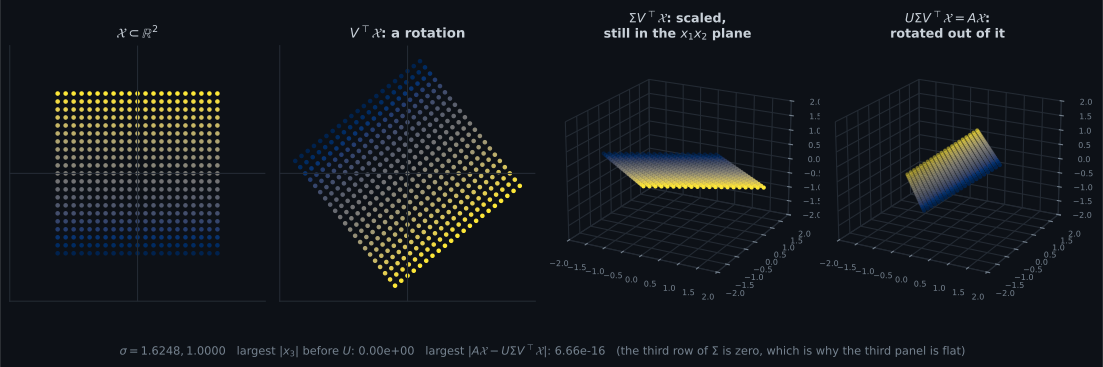
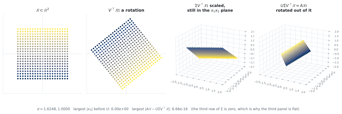
Reading the plot

From the three-stage figure. Follow the two coloured vectors, not the cloud. In the first panel they are $\mathbf{v}_1$ and $\mathbf{v}_2$, at some oblique angle to the axes. In the second they lie on the axes — that is all $\mathbf{V}^\top$ does. In the third they have been stretched by $1.6248$ and $1$ and the whole grid now lives in $\mathbb{R}^3$, but flatly: max |x3| = 0.00e+00. The fourth panel is the only one where the disc leaves the plane.

The number worth staring at is that exact zero. It is not $10^{-16}$; it is zero, because $\boldsymbol{\Sigma}$‘s third row contains no nonzero entry that could put anything there. The change of dimension in the SVD is a padding, not a computation.

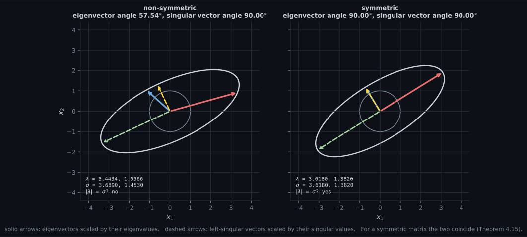
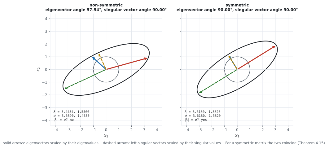
From the eigen-versus-singular figure. The left panel corrects a common misconception. For the non-symmetric $[[3, 1.6], [0.4, 2]]$:

	first	second	the pair’s angle
eigenvalues, along invariant directions	$3.4434$	$1.5566$	$57.54°$
singular values, along orthogonal directions	$3.6890$	$1.4530$	$90.00°$

These are different numbers, and neither is a rounding of the other. The eigenvalues say how much the matrix stretches along its two invariant directions; the singular values say how much it stretches along its two orthogonal directions of greatest and least stretch. Those are different questions, and they have the same answer only when the invariant directions happen to be orthogonal.

The angle column is the mechanism. The singular vectors meet at exactly $90°$ always — that is what ”$\mathbf{U}$ is orthogonal” means, and it is not an accident of this matrix. The eigenvectors meet at $57.54°$ here, so they cannot possibly be the axes of an ellipse. The right panel makes the matrix symmetric and the eigenvector angle becomes $90°$; at that moment both spectra read $3.6180$ and $1.3820$, identical to every printed digit.

One quantity survives either way: $\lvert\det\mathbf{A}\rvert = 5.36$ and $\sigma_1\sigma_2 = 3.6890 \times 1.4530 = 5.36$. Both factorisations agree about volume even when they disagree about every individual factor.

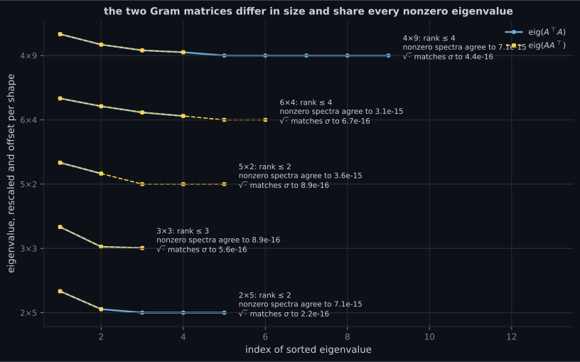
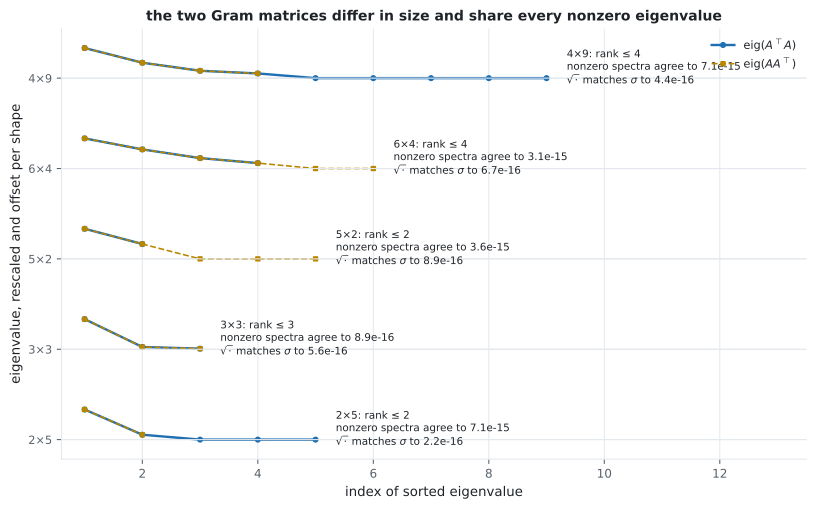
From the Gram figure. Read it one row at a time; each row is one matrix shape, and the two curves are the sorted spectra of the two Gram matrices. They lie on top of each other. Across the five shapes the nonzero spectra agree to at most $7.1\times10^{-15}$ and their square roots match the singular values to at most $8.9\times10^{-16}$.

The detail the figure adds is what happens to the extra eigenvalues, and the $4\times9$ row shows it best: $\mathbf{A}^\top\mathbf{A}$ is $9\times9$ with nine eigenvalues while $\mathbf{A}\mathbf{A}^\top$ is only $4\times4$ with four. Four of them match; the other five are zero. Those five zeros are the kernel of $\mathbf{A}$, and their eigenvectors are the last five columns of $\mathbf{V}$ — the free null-space basis from Equation 4.79.

Note also that the two Gram matrices are different sizes and still share a spectrum apart from zeros. That is what makes the construction work from either end: you can build $\mathbf{V}$ from the smaller one and get the same $\sigma_i$.

Pitfalls

Never compute an SVD through the Gram matrix in production

The book says so at Equation 4.88 and the reason is conditioning: $\kappa(\mathbf{A}^\top\mathbf{A}) = \kappa(\mathbf{A})^2$. Measured on a $6\times4$ with a prescribed spectrum, the relative error in the smallest singular value runs $1.2\times10^{-14}$, $2.4\times10^{-9}$, $4.2\%$, then $100\%$ as $\kappa(\mathbf{A})$ goes $10^2$, $10^4$, $10^8$, $10^{12}$ — at the end the Gram route returns exactly zero. And there is a second, subtler failure: the square root halves the exponent, so a rounding error at $10^{-16}$ in the Gram matrix becomes a spurious singular value at $10^{-8}$, which is what makes the rank-1 example above come back with the wrong rank. The construction is a proof, not an algorithm. Use np.linalg.svd, which reduces to bidiagonal form and never forms the Gram.

Singular values are not the absolute values of the eigenvalues

Measured on $[[4,2],[1,3]]$: eigenvalues $5$ and $2$, singular values $5.116673$ and $1.954395$. On the figure’s $[[3,1.6],[0.4,2]]$: $3.4434$ and $1.5566$ against $3.6890$ and $1.4530$. The identity $\sigma_i = \lvert\lambda_i\rvert$ holds only for symmetric matrices. What always holds is $\prod\sigma_i = \lvert\det\mathbf{A}\rvert$ and $\sigma_1 = \lVert\mathbf{A}\rVert_2$.

The signs of the singular vectors are arbitrary

Only the pairs are determined. Flipping $\mathbf{u}_i$ and $\mathbf{v}_i$ together leaves $\mathbf{A}$ unchanged, so different libraries, versions and platforms return different signs — and the book’s own Figure 4.10 differs from np.linalg.svd in the sign of the third singular vector for exactly this reason. Never read a sign as meaning anything; compare $\lvert\mathbf{U}\rvert$ or fix a convention yourself (for instance, force the largest-magnitude entry of each column positive).

full_matrices=True is the default and is usually not what you want

For a $10000\times50$ matrix the default asks for a $10000\times10000$ $\mathbf{U}$ — eight hundred megabytes to hold $9950$ columns you will never use. Pass full_matrices=False unless you specifically need a basis for the orthogonal complement.

Repeated singular values make the singular vectors non-unique

If $\sigma_i = \sigma_{i+1}$ then any rotation within that two-dimensional subspace gives an equally valid pair of singular vectors, so individual columns are meaningless. The second sketch above shows it: set $a_{12} = a_{21} = 0$ with $a_{11} = a_{22}$ and both singular values become equal, at which point $\mathbf{v}_1$ and $\mathbf{v}_2$ stop being determined at all.

Σ is not square, and neither is its “inverse”

$\boldsymbol{\Sigma}$ has the shape of $\mathbf{A}$. You cannot write $\boldsymbol{\Sigma}^{-1}$; the pseudo-inverse is $\boldsymbol{\Sigma}^{+}$, formed by transposing and reciprocating only the nonzero entries. np.linalg.pinv does this, and it is where Chapter 9’s least-squares solution comes from.

Compare

decomposition	hypothesis	outer factors	middle	what it is for
LU	none (with pivoting)	triangular	—	solving systems, determinants
Cholesky $\mathbf{L}\mathbf{L}^\top$	symmetric positive definite	triangular, and each other’s transpose	—	sampling, fast determinants, §4.3
QR	none	orthogonal, triangular	—	least squares without forming a Gram
eigendecomposition $\mathbf{P}\mathbf{D}\mathbf{P}^{-1}$	square, non-defective	invertible, inverse to each other	may be negative or complex	matrix powers, §4.4
SVD $\mathbf{U}\boldsymbol{\Sigma}\mathbf{V}^\top$	none	orthogonal, in different spaces	real, non-negative	rank, all four subspaces, pseudo-inverse, best low-rank approximation

pch.quizTag Check your understanding

1. Why can U and V not be inverses of each other, the way P and P-inverse are?

   A They can be, for square matrices B Because they perform basis changes in different vector spaces — U is m by m in the codomain and V is n by n in the domain, so their product is not even defined in general C Because they are orthogonal D Because Sigma is not square
   pch.quizShowAnswer

   B — Because they perform basis changes in different vector spaces — U is m by m in the codomain and V is n by n in the domain, so their product is not even defined in general — This is the structural difference the book highlights in §4.5.3. The eigendecomposition applies one basis change and then undoes it inside one space; the SVD links two different bases in two different spaces through Sigma.

2. For the matrix [[4,2],[1,3]] the eigenvalues are 5 and 2 while the singular values are 5.116673 and 1.954395. What went wrong?

   A A rounding error in one of the two computations B Nothing. The identity sigma-i equals the absolute value of lambda-i holds only for symmetric matrices; eigenvalues measure stretch along invariant directions and singular values measure stretch along orthogonal ones C The matrix is defective D The singular values were computed from the wrong Gram matrix
   pch.quizShowAnswer

   B — Nothing. The identity sigma-i equals the absolute value of lambda-i holds only for symmetric matrices; eigenvalues measure stretch along invariant directions and singular values measure stretch along orthogonal ones — What does survive is the product: 5.116673 times 1.954395 is exactly 10, which is the absolute determinant. Both factorisations agree about volume while disagreeing about the individual factors.

3. In the three-stage figure, the third coordinate after Sigma is measured as exactly 0.00e+00 rather than something near 1e-16. Why exactly zero?

   A A lucky cancellation B Because the bottom row of Sigma is all zeros, so there is no arithmetic that could put a nonzero value in the third coordinate — the change of dimension is a padding, not a computation C Because the matrix is orthogonal D Because the grid was chosen to make it so
   pch.quizShowAnswer

   B — Because the bottom row of Sigma is all zeros, so there is no arithmetic that could put a nonzero value in the third coordinate — the change of dimension is a padding, not a computation — That is the whole content of Equations 4.65 and 4.66. Sigma has the shape of A and pads with zeros, so it can lift into a higher dimension only by putting zeros there. Only U tilts anything out of that plane.

4. The book states the Gram construction and then immediately warns against using it. Why?

   A It is slower B Because forming A-transpose A squares the condition number, so at a condition number of 1e8 — routine for a design matrix — the Gram matrix is numerically singular in double precision and the small singular values are destroyed C Because eigh does not exist for all matrices D Because it gives the wrong signs
   pch.quizShowAnswer

   B — Because forming A-transpose A squares the condition number, so at a condition number of 1e8 — routine for a design matrix — the Gram matrix is numerically singular in double precision and the small singular values are destroyed — The from-scratch implementation on this page shows a symptom of the same disease: eigh returns a tiny negative eigenvalue where zero was expected, and without clipping it np.sqrt produces nan.

5. For a 3x5 matrix of rank 3, what do the last two columns of V give you?

   A Nothing; they are padding B An orthonormal basis of the kernel of A, since A v-i equals zero for those columns while they remain orthonormal by construction C The left-singular vectors D The eigenvectors of A
   pch.quizShowAnswer

   B — An orthonormal basis of the kernel of A, since A v-i equals zero for those columns while they remain orthonormal by construction — The book makes the point right after Equation 4.79: where the singular value equation says nothing, the vectors are still orthonormal, so the SVD hands you a basis for the null space for free.

🧪 Try It Yourself

Exercise 1 – Example 4.13, the construction in three steps

pch.exerciseTag pch.exerciseTitle

Exercise 2 – Sigma has the shape of A

pch.exerciseTag pch.exerciseTitle

Exercise 3 – Eigenvalues against singular values

pch.exerciseTag pch.exerciseTitle

Exercise 4 – The kernel, for free

pch.exerciseTag pch.exerciseTitle

Exercise 5 – Why the Gram route is a proof and not an algorithm

pch.exerciseTag pch.exerciseTitle

Recall card

• The SVD has no hypothesis: A equals U Sigma V-transpose for every real matrix of every shape, which is why it is called the fundamental theorem of linear algebra.
• Both outer matrices are orthogonal, and Sigma has the shape of A — rectangular, with zero padding below or to the right, and real non-negative diagonal entries in descending order.
• U and V change basis in different spaces, so unlike P and P-inverse they are not inverses of each other; Sigma is what links the two bases.
• The geometry is rotate, scale-and-change-dimension, rotate. The change of dimension is a padding: after Sigma the extra coordinates are exactly zero, not merely small.
• V comes from the eigenvectors of A-transpose A and U from those of A A-transpose, with the squared singular values as the shared nonzero eigenvalues of both.
• The singular value equation is A v-i = sigma-i u-i, which resembles the eigenvalue equation except that the two sides involve different vectors.
• The trailing columns of V are an orthonormal basis of the kernel, so the SVD hands you the null space for free.
• Never compute an SVD through the Gram matrix: it squares the condition number — the smallest singular value is 4 percent wrong at kappa 1e8 and lost entirely at 1e12 — and the square root halves the exponent, turning a 1e-16 rounding error into a spurious 1e-8 singular value that breaks the rank test.
• Singular values are the absolute eigenvalues only for symmetric matrices. For [[4,2],[1,3]] the eigenvalues are 5 and 2 while the singular values are 5.116673 and 1.954395; what always holds is that their product is the absolute determinant.
• For a symmetric matrix the eigendecomposition and the SVD are the same thing, which follows from the spectral theorem and is why PCA can be described either way.

Next: Matrix Approximation — truncate the sum and you get the provably closest low-rank matrix, with the error known in advance.