Responsibilities

Page 1102 ended with the same factor appearing in every derivative: $\pi_k\mathcal{N}(\mathbf{x}_n\mid\cdot)$ over the whole mixture density. §11.2.1 gives it a name and a meaning, and the book flags how much work it will do:

But before we do this, we introduce a quantity that will play a central role in the remainder of this chapter: responsibilities.

What you’ll learn

Equation 11.17’s definition, and Equation 11.19 checked entry by entry — including one place the book’s printed matrix disagrees with the arithmetic, by $0.001$ .
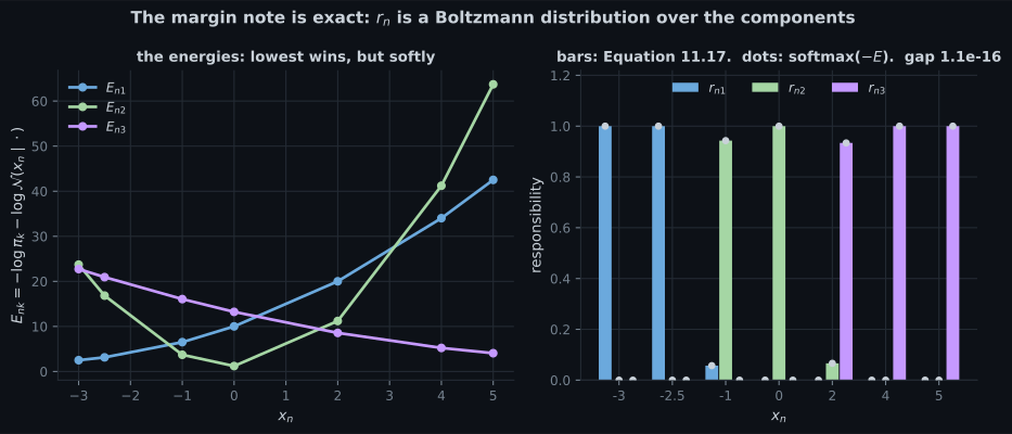
Equation 11.24: $N_k = \sum_n r_{nk}$ , and $\sum_k N_k = N$ to $7.000000000000$ .
The margin note ” $\mathbf{r}_n$ follows a Boltzmann/Gibbs distribution”, verified: $\mathbf{r}_n = \mathrm{softmax}(-\mathbf{E}_n)$ with $E_{nk} = -\log\pi_k - \log\mathcal{N}(x_n\mid\mu_k,\sigma_k^2)$ , matching to $1.1\times10^{-16}$ .
What “soft assignment” buys on this data: at the initialisation the least-decided point is $x = 2$ at $0.933753$ ; at convergence it is $x = 0$ at $0.983469$ .
The entropy of $\mathbf{r}_n$ as a measure of how much softness is actually in play — mean $0.066338$ at the start against a maximum of $\log 3 = 1.098612$ .
Shrink every variance and the responsibilities become indicator vectors — which is K-means, exactly as §11.5 says.
And a practical trap: Equation 11.17 typed out as written produces $21$ NaNs of $21$ entries once the variances are small; in log-space it produces the exact one-hot answer.

Intuition: a soft assignment is the only thing that can be differentiated

Suppose you knew which component made each point. Then fitting is trivial — split the data and fit each Gaussian to its own share, with the closed forms of Chapter 8. That is the whole difficulty: you do not know.

The obvious repair is to guess — assign each point to its most likely component and fit. That is K-means, and it works, but it throws away the fact that some points are genuinely ambiguous. Worse, it is not differentiable: nudge a parameter and a point’s label jumps discontinuously.

The responsibility is the repair that keeps the calculus. Each point contributes to every component, weighted by how plausible that component makes it. Nothing jumps, everything differentiates, and the hard assignment reappears as a limit.

diagram Where the responsibility comes from and what it becomes mermaid

  flowchart TD
  A["1 / p(x_n | theta) in every derivative
Equation 11.16"]
  A --> B["r_nk = pi_k N(x_n | k) / sum_j pi_j N(x_n | j)
Equation 11.17"]
  B --> C["a probability vector: sums to 1"]
  B --> D["N_k = sum_n r_nk
Equation 11.24"]
  D --> E["mu_k, Sigma_k, pi_k updates
Sections 11.2.2 to 11.2.4"]
  B --> F["posterior p(z_nk = 1 | x_n)
Section 11.4.3"]
  B --> G["variances to 0: one-hot
= K-means, Section 11.5"]

§11.2.1 The definition

r_{nk} := \frac{\pi_k\mathcal{N}(\mathbf{x}_n\mid\boldsymbol\mu_k,\boldsymbol\Sigma_k)}{\sum_{j=1}^{K}\pi_j\mathcal{N}(\mathbf{x}_n\mid\boldsymbol\mu_j,\boldsymbol\Sigma_j)} \qquad \text{(11.17)}

The responsibility $r_{nk}$ of the $k$ th mixture component for data point $\mathbf{x}_n$ is proportional to the likelihood […] Therefore, mixture components have a high responsibility for a data point when the data point could be a plausible sample from that mixture component.

$\mathbf{r}_n = [r_{n1},\ldots,r_{nK}]^\top$ is a normalised probability vector, $\sum_k r_{nk} = 1$ with $r_{nk} \geq 0$ — a “soft assignment” of $\mathbf{x}_n$ to the $K$ components.

Top, two seven-by-three heat maps of responsibilities, mostly bright yellow or dark purple with a few intermediate cells, labelled with their values. Bottom, a stacked area chart across the real line in three colours summing to one everywhere, with seven red triangular markers showing the data. — Each row of the heat maps sums to 1. The bottom panel is the converged model's responsibilities as continuous functions of x — they partition the line, and the transitions between components are smooth rather than abrupt, which is exactly what makes them differentiable.

Computed at the book’s own initialisation, to six decimals:

$x_n$	$r_{n1}$	$r_{n2}$	$r_{n3}$	the book’s row
$-3.0$	$1.000000$	$0.000000$	$0.000000$	$[1, 0, 0]$
$-2.5$	$0.999999$	$0.000001$	$0.000000$	$[1, 0, 0]$
$-1.0$	$0.057069$	$0.942926$	$0.000004$	$[0.057, 0.943, 0]$
$\mathbf{0.0}$	$\mathbf{0.000150}$	$\mathbf{0.999844}$	$0.000006$	$\mathbf{[0.001, 0.999, 0]}$
$2.0$	$0.000010$	$0.066237$	$0.933753$	$[0, 0.066, 0.934]$
$4.0$	$0.000000$	$0.000000$	$1.000000$	$[0, 0, 1]$
$5.0$	$0.000000$	$0.000000$	$1.000000$	$[0, 0, 1]$

Every row matches to the printed precision except the fourth: $0.000150$ rounds to $0.000$ , not $0.001$ , and $0.999844$ rounds to $1.000$ , not $0.999$ . The largest disagreement is $0.001$ — a typo or a rounding choice, not a mathematical error, and it changes nothing downstream. Worth knowing if you check your own implementation against the printed matrix.

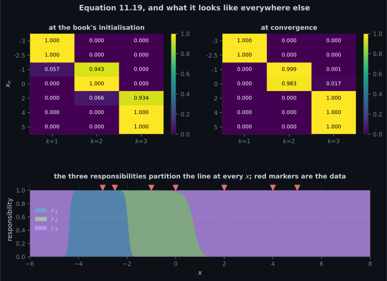
The book’s reading of the matrix does hold: “the third mixture component is not responsible for any of the first four data points” — measured, its largest responsibility among those four is $6.0\times10^{-6}$ .

Summing down the columns gives Equation 11.24:

N_k := \sum_{n=1}^{N} r_{nk} \qquad \text{(11.24)}

	$k=1$	$k=2$	$k=3$	total
$N_k$ at the initialisation	$2.057228$	$2.009008$	$2.933763$	$\mathbf{7.000000000000}$

$N_k$ is a count that need not be a whole number — the effective number of points each component owns. That it sums to $N$ exactly is the column-sum counterpart of the rows summing to $1$ , and it is what makes Equation 11.42’s $\pi_k = N_k/N$ a valid set of weights.

The margin note, checked

$\mathbf{r}_n$ follows a Boltzmann/Gibbs distribution.

Write $E_{nk} := -\log\pi_k - \log\mathcal{N}(x_n\mid\mu_k,\sigma_k^2)$ . Then Equation 11.17 is exactly

r_{nk} = \frac{e^{-E_{nk}}}{\sum_j e^{-E_{nj}}} = \mathrm{softmax}(-\mathbf{E}_n)_k

Measured, $\max\lvert\mathrm{softmax}(-\mathbf{E}) - \mathbf{r}\rvert = 1.1\times10^{-16}$ .

Left, three lines of energy against data point, crossing each other so that a different one is lowest in each of three regions. Right, grouped bars of responsibility with a small dark dot sitting exactly on top of every bar. — On the left the lowest energy wins — but softly, because the gap matters, not just the order. At x = -1 the first two energies are 6.5176 and 3.7128, a gap of 2.8, giving 0.057 against 0.943. The dots on the right are the softmax of the negated energies; they land on the bars to 1.1e-16.

Three things follow immediately from softmax over energies, and each reappears later:

The gap is what matters, not the ranking. $r_{n1}/r_{n2} = e^{E_{n2}-E_{n1}}$ , so a component two nats better takes about $7.4$ times the responsibility regardless of what the other energies are.

The prior enters as an offset. $-\log\pi_k$ shifts a component’s energy uniformly in $x$ , so changing the mixture weights slides responsibility without changing where the boundaries are shaped — which is why page 1106’s weight update is the simplest of the three.

Temperature is variance. Scaling every $\sigma_k^2$ by $t$ scales the quadratic part of every energy by $1/t$ , which is a Boltzmann distribution at temperature $t$ . That is the next section.

Soft, and how soft

On the book’s seven points, soft assignment is barely being used:

	least-decided point	its $\max_k r_{nk}$	points below $0.9$	mean entropy
at the initialisation	$x = 2$	$0.933753$	$0$ of $7$	$0.066338$
at convergence	$x = 0$	$0.983469$	$0$ of $7$	$0.013865$

against a maximum possible entropy of $\log 3 = 1.098612$ . Seven well-separated points in one dimension do not need much softness — but the algorithm does, because a hard assignment is not differentiable, and because the book’s own Figure 11.10(b) shows the opposite case: “the responsibilities of these two clusters for those points are around $0.5$ .”

Turn the temperature down and you get K-means

Scaling every variance by $t$ and letting $t \to 0$ :

$t$	mean $\max_k r_{nk}$	mean entropy	points above $0.99$
$10^{2}$	$0.513458$	$0.943042$	$0$
$10^{1}$	$0.793531$	$0.514462$	$1$
$10^{0}$	$0.997409$	$0.013865$	$6$
$10^{-1}$	$1.000000$	$0.000000$	$7$
$10^{-6}$	$\mathbf{1.000000}$	$\mathbf{0.000000}$	$\mathbf{7}$

Left, a blue curve rising from about 0.5 to 1 and an amber curve falling from near 1 to 0 as the variance scale decreases, with dotted guide lines at one and one third. Right, a red curve that is flat at zero and then jumps to 21, against a blue dashed line that stays at zero throughout. — Left: at large variances every component is equally plausible and the responsibilities approach 1/K; at small variances they become indicator vectors, which is K-means. Right: the naive form of Equation 11.17 computes zero over zero once the densities underflow, returning NaN for all 21 entries, while the log-space form returns the exact one-hot answer.

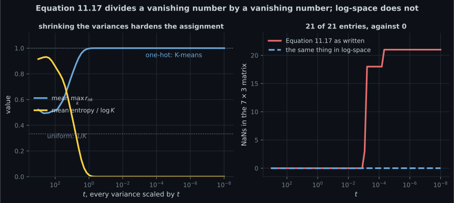
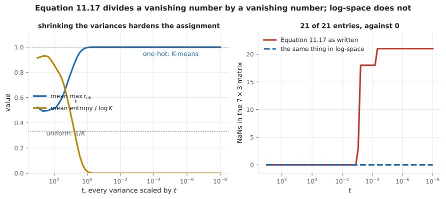
§11.5 states the relationship: “If we treat the means in the GMM as cluster centers and ignore the covariances (or set them to $\mathbf{I}$ ), we arrive at K-means. […] K-means makes a ‘hard’ assignment of data points to cluster centers, whereas a GMM makes a ‘soft’ assignment via the responsibilities.”

On this data, run from the book’s own starting means, the two do not land in the same place:

	centres	cluster sizes	within-cluster SS
GMM at convergence	$-2.750036,\ -0.504119,\ 3.644573$	$1.982478,\ 1.999703,\ 3.017819$	—
K-means from $[-4, 0, 8]$	$-2.166667,\ 1.000000,\ 4.500000$	$3, 2, 2$	$\mathbf{4.666667}$
K-means handed the GMM’s answer	$-2.750000,\ -0.500000,\ 3.666667$	$2, 2, 3$	$5.291667$

Two things worth separating. From the same start the two algorithms disagree by $1.504119$ — they split the seven points differently, $3\!-\!2\!-\!2$ against effectively $2\!-\!2\!-\!3$ . And the GMM’s partition is not even the better K-means answer: its within-cluster sum of squares is $5.291667$ against $4.666667$ .

The reason is in the last row of the GMM’s parameters: its variances are $0.0625$ , $0.250581$ and $1.628941$ — a factor of $26.06$ apart. K-means has no variances, so it cannot prefer a tight cluster of two over a loose cluster of three. Only if you hand K-means the GMM’s own answer does it stay there, and then the centres agree to $0.022094$ and the counts differ only by being integers.

The numerator and denominator both underflow long before the ratio does. Measured on the converged model with every variance scaled by $t$ :

$t$	NaNs from Equation 11.17 as written	NaNs in log-space
$10^{-2}$	$0$	$0$
$10^{-3}$	$3$	$0$
$10^{-6}$	$\mathbf{21}$ of $21$	$\mathbf{0}$

The fix is the same one every implementation uses: form $\log\pi_k + \log\mathcal{N}(x_n\mid\cdot)$ , subtract the row’s logsumexp, and exponentiate. Where both work they agree to $2.2\times10^{-16}$ .

This is not a small-variance curiosity. In $D$ dimensions the log-density scales with $D$ , so a well-conditioned model on $784$ -pixel images hits the same underflow at perfectly ordinary parameter values.

pch.quizTag Are responsibilities clear?

What is r_nk, in one sentence?

pch.quizShowAnswer

B — The share of x_n that component k is credited with — its weighted density over the whole mixture's density at that point — Equation 11.17. Each row sums to one, so it is a probability vector over components — a soft assignment. Section 11.4.3 later identifies it as a genuine posterior, the probability that the k-th component generated the n-th point.
The book's margin note calls r_n a Boltzmann distribution. Is that exact?

pch.quizShowAnswer

B — It is exact: r_n is the softmax of minus the energies -log pi_k - log N(x_n | k), matching to 1.1e-16 — And the framing pays: the ratio of two responsibilities is the exponential of their energy gap, the mixture weight enters as a uniform offset, and scaling all the variances by t is exactly a temperature. The last of those is the K-means limit.
What is N_k, and why need it not be a whole number?

pch.quizShowAnswer

B — The column sum of the responsibilities — an effective count, fractional because the assignment is soft, summing to N exactly — Measured at the book's initialisation: 2.057228, 2.009008 and 2.933763, summing to 7.000000000000. K-means from the same start gives integer sizes 3, 2 and 2 — a different split entirely, because it has no variances with which to prefer a tight cluster over a loose one.
What goes wrong if you code Equation 11.17 exactly as printed?

pch.quizShowAnswer

B — Numerator and denominator both underflow to zero, giving NaN — all 21 entries of a 7-by-3 matrix once the variances are small — The fix is to work in log-space: add the log weight to the log density, subtract the row's logsumexp, exponentiate. Where both forms work they agree to 2.2e-16. This is not exotic — in D dimensions the log-density scales with D, so 784-pixel images hit it at ordinary parameter values.

Exercises

Exercise 1 – Check Equation 11.19 against the arithmetic

Exercise 2 – The margin note, as arithmetic

Exercise 3 – How much softness is actually used

Exercise 4 – Turn the temperature down

Exercise 5 – Soft counts against hard counts

Recall card

The responsibility is the factor that appeared in every derivative on the previous page, given a name: component k’s weighted density at a point, over the whole mixture’s density there.
Each row is a probability vector, so responsibilities are a soft assignment of a point to the components.
Summing down a column gives N_k, the effective number of points a component owns — fractional, and summing to N exactly.
The book’s printed responsibility matrix disagrees with the arithmetic at one entry, by 0.001; the computed value at x equal to zero is 0.000150, not 0.001.
The margin note is exact, not a metaphor: the responsibility vector is the softmax of minus the energies, matching to 1.1e-16.
So the ratio of two responsibilities is the exponential of their energy gap, the mixture weights enter as a uniform offset, and the variances act as a temperature.
On the book’s seven points the softness is barely used — mean entropy 0.014 at convergence against a possible 1.099 — because the clusters are well separated.
Shrinking every variance drives the responsibilities to indicator vectors, which is K-means. Section 11.5 says exactly this.
But from the same starting means they do not agree: centres 1.504119 apart, splitting the points 3-2-2 against effectively 2-2-3, because K-means has no variances to weigh a tight cluster against a loose one.
Equation 11.17 typed out as written divides a vanishing number by a vanishing number, returning NaN for all 21 entries once the variances are small.
In log-space it returns the exact answer, and where both work they agree to 2.2e-16.
A hard assignment is not a rounding of a soft one — it is a different algorithm, and the soft version is the one that can be differentiated.

Next: Updating the Means — §11.2.2, the first of three updates, and the one the book draws a picture for.

pch.coffeeTagline

pch.coffeeCta

pch.feedbackHeading

pch.feedbackSubheading