What you’ll learn

• how an ROC curve is constructed, one threshold at a time
• the full curve traced by hand from the ten-row example
• the probabilistic meaning of AUC — it is not “accuracy over all thresholds”
• why AUC = 0.5 is chance and AUC below 0.5 means something useful
• exactly when ROC misleads, and why precision-recall is the right choice there
• how to pick between ROC-AUC and average precision, with a rule

Intuition

Precision and recall describe one operating point. The ROC curve describes all of them at once.

Slide the threshold from 1 down to 0. At the top, nothing is predicted positive: no true positives, no false positives, and the curve starts at $(0, 0)$. At the bottom, everything is predicted positive and the curve ends at $(1, 1)$. In between, every threshold contributes a point.

The shape of the path between those corners is the model’s ranking ability. A model that scores every positive above every negative goes straight up and then straight across — through the top-left corner. A model that ranks randomly follows the diagonal.

  flowchart LR
  A["Sort all predictions
by score, descending"] --> B["Walk down the list"]
  B --> C{"Is this row
actually positive?"}
  C -->|yes| U["Step up
TPR increases"]
  C -->|no| R["Step right
FPR increases"]
  U --> B
  R --> B

The math

Both denominators are row totals of the confusion matrix — the number of actual positives and the number of actual negatives. That single fact explains everything ROC does well and everything it does badly: neither axis depends on how many positives there are relative to negatives, so the curve is invariant to class balance.

What AUC actually measures

The area under the ROC curve has an exact probabilistic interpretation:

AUC is the probability that a randomly chosen positive is ranked above a randomly chosen negative. It is a measure of ranking, not of classification. It never looks at your threshold, which is exactly why it is useful for comparing models before one is chosen — and why it cannot tell you whether a model is deployable.

That last row is worth remembering. An AUC of 0.2 is not a bad model, it is a good model with its labels or its sign the wrong way round.

Worked example by hand

The ten-row example, sorted by score. Five positives, five negatives.

Each row is one threshold. A positive steps the curve up by $1/5$; a negative steps it right by $1/5$.

Area by geometry. The curve is a staircase, so the area is a sum of rectangles — one per rightward step, whose height is the TPR at that moment:

Area by counting pairs. The probabilistic definition gives the same answer directly. There are $5 \times 5 = 25$ positive/negative pairs; count how many the model ranks correctly:

Two completely different routes, the same number — and roc_auc_scoreroc_auc_score returns exactly 0.84. The pair-counting view is the one worth carrying: AUC is the fraction of positive/negative pairs your model gets in the right order.

See it move

The sketch draws both routes at once. On the left, the ranked list is consumed one row at a time and the staircase is built step by step — up for a positive, right for a negative, with the rectangle under each rightward step shaded as it is added. On the right, the same event is scored as pairs: the $5 \times 5$ grid fills in green for each correctly ordered pair. The two totals stay equal throughout.

The four red cells in the grid are the model’s entire mistake: score 0.58 and 0.31 each lose to the negatives at 0.70 and 0.62. Twenty-one of twenty-five pairs are ordered correctly, and the staircase area is the same 0.84 because each rectangle is exactly the set of pairs resolved by that rightward step. The equivalence is not a coincidence to memorise; it is the same count, grouped two different ways.

On real data

figureROC on a balanced problem, and the imbalanced case where it misleadsmatplotlib

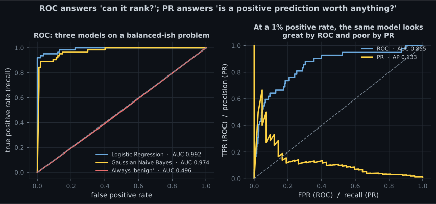
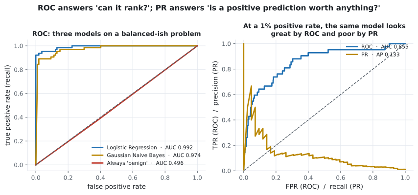
Reading the plot

Left panel — a healthy comparison.

• Logistic regression reaches AUC 0.992, Naive Bayes 0.974. Both are strong; the ranking between them is what AUC is for.
• The random classifier lands on 0.496 — the diagonal, within sampling noise of exactly 0.5.
• The steep initial rise matters most: it means the highest-scoring predictions are almost all genuine positives, which is what you exploit when you can only act on the top few.

Right panel — the failure mode.

• Positive rate is 1%. ROC-AUC reports 0.855, which sounds like a good model.
• Average precision reports 0.133.
• Both are computed from identical predictions. The disagreement is not a bug; it is the two metrics answering different questions.

Why ROC is optimistic under imbalance

FPR has $TN$ in its denominator, and under heavy imbalance $TN$ is enormous. With 3,960 negatives and 40 positives, 200 false positives give:

which barely moves the curve. But those same 200 false positives destroy precision:

ROC absorbs false positives into a huge negative pool; precision does not, because it never counts true negatives at all. When the positive class is rare, precision is measuring the thing you actually care about — is a flag worth investigating? — and ROC is not.

Multiclass ROC

ROC is defined for binary problems. For $K$ classes, compute one curve per class one-versus-rest and average:

from sklearn.datasets import load_digits
from sklearn.linear_model import LogisticRegression
from sklearn.metrics import roc_auc_score
from sklearn.model_selection import train_test_split
from sklearn.pipeline import make_pipeline
from sklearn.preprocessing import StandardScaler
 
digits = load_digits()
X_tr, X_te, y_tr, y_te = train_test_split(
    digits.data, digits.target, test_size=0.3, random_state=0, stratify=digits.target
)
 
model = make_pipeline(StandardScaler(), LogisticRegression(max_iter=5000))
model.fit(X_tr, y_tr)
proba = model.predict_proba(X_te)
 
macro = roc_auc_score(y_te, proba, multi_class="ovr", average="macro")
weighted = roc_auc_score(y_te, proba, multi_class="ovr", average="weighted")
 
print(f"macro OvR AUC    {macro:.4f}")      # 0.9992
print(f"weighted OvR AUC {weighted:.4f}")   # 0.9992

from sklearn.datasets import load_digits
from sklearn.linear_model import LogisticRegression
from sklearn.metrics import roc_auc_score
from sklearn.model_selection import train_test_split
from sklearn.pipeline import make_pipeline
from sklearn.preprocessing import StandardScaler
 
digits = load_digits()
X_tr, X_te, y_tr, y_te = train_test_split(
    digits.data, digits.target, test_size=0.3, random_state=0, stratify=digits.target
)
 
model = make_pipeline(StandardScaler(), LogisticRegression(max_iter=5000))
model.fit(X_tr, y_tr)
proba = model.predict_proba(X_te)
 
macro = roc_auc_score(y_te, proba, multi_class="ovr", average="macro")
weighted = roc_auc_score(y_te, proba, multi_class="ovr", average="weighted")
 
print(f"macro OvR AUC    {macro:.4f}")      # 0.9992
print(f"weighted OvR AUC {weighted:.4f}")   # 0.9992

macromacro treats every class equally and weightedweighted scales by support — the same choice as for multiclass F1, and the same advice: with imbalanced classes, macromacro is usually the honest one.

ROC-AUC versus average precision

The invariance is genuinely a feature and genuinely a bug, depending on the question. If you are comparing two models on the same data, invariance is helpful. If you are deciding whether a fraud model is worth deploying, invariance hides the fact that 87% of its alerts are wrong.

Pitfalls

🧪 Try It Yourself

Exercise 1 – Compute one point on the curve

Exercise 2 – Trace the whole curve

Exercise 3 – AUC by counting pairs

Exercise 4 – Spot a near-random classifier

Exercise 5 – Watch ROC and AP disagree

Recap

• The ROC curve sweeps every threshold, plotting TPR against FPR; both denominators are row totals, so the curve is invariant to class balance.
• Each positive steps the curve up, each negative steps it right.
• AUC is $P(\text{positive scores above negative})$ — a ranking statistic. The ten-row example gives 21 of 25 correctly ordered pairs, so AUC = 0.84 by geometry and by counting.
• 0.5 is chance; below 0.5 means the ranking is inverted, not that the model is worthless.
• Under heavy imbalance, ROC is optimistic because FPR hides false positives in a huge negative pool. The same predictions scored 0.855 by ROC and 0.133 by average precision.
• Balanced or symmetric costs → ROC-AUC. Rare positives you act on → average precision.

Exercise 6 – The same 0.84, computed three ways

Next

Phase 4 ends here. Continue to Phase 5 - Ensemble Learning — where the instability of a single decision tree, noted at the end of the trees page, becomes the foundation of the strongest models in classical machine learning.