
Handling Text & Categorical Attributes
What you’ll learn
Section titled “What you’ll learn”- why
OrdinalEncodermakes a claim about your data, and when that claim is false - one-hot encoding, and the geometric reason it is the safe default
- the memory arithmetic behind sparse matrices — 20,640 × 5 stored in 165 KB or 826 KB
- the dummy variable trap, and when
drop="first"matters and when it does not - what happens when an unseen category arrives in production
- four alternatives for high-cardinality columns, with the cost of each
Intuition
Section titled “Intuition”Almost no model accepts the string "NEAR BAY". Encoding turns text into numbers, and the encoding
you pick is not a formatting decision — it tells the model what it is allowed to believe about
those categories.
Map five categories to 0–4 and you have asserted that they lie on a line, evenly spaced, in that
order. Sometimes true (small < medium < large). Here, false: ISLAND is not “between” INLAND
and NEAR BAY in any sense, yet a linear model will treat the numbers exactly that way.
  flowchart LR
  T["Text column"] --> Q{"Do the categories
have a real order?"}
  Q -->|yes| O["OrdinalEncoder
1 column, ordering preserved"]
  Q -->|no| C{"How many
distinct values?"}
  C -->|"under ~50"| H["OneHotEncoder
one column each"]
  C -->|"hundreds or more"| A["Target / frequency /
hashing / embedding"]
The one text column
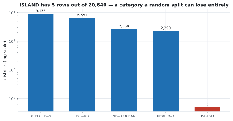
Section titled “The one text column”print(housing["ocean_proximity"].value_counts())
# <1H OCEAN 9136
# INLAND 6551
# NEAR OCEAN 2658
# NEAR BAY 2290
# ISLAND 5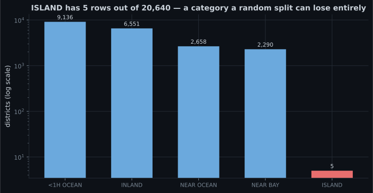
Ordinal encoding
Section titled “Ordinal encoding”from sklearn.preprocessing import OrdinalEncoder
encoder = OrdinalEncoder()
encoded = encoder.fit_transform(housing[["ocean_proximity"]])
print(encoder.categories_)
# [array(['<1H OCEAN', 'INLAND', 'ISLAND', 'NEAR BAY', 'NEAR OCEAN'], dtype=object)]
print(encoded[:5].ravel()) # [3. 3. 3. 3. 3.]Categories are assigned integers in alphabetical order, which is where the trouble starts.
ISLAND becomes 2 purely because “I” sorts between “I” and “N” — and a linear model then reads
that as: an island district is numerically between an inland one and a bay one, and twice as far
from <1H OCEAN as INLAND is.
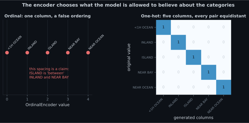
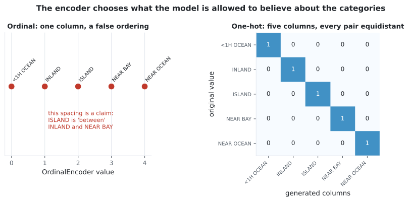
Geometrically: under one-hot every pair of categories is apart, so no ordering and no spacing is implied. Under ordinal the distances are 1, 2, 3 and 4, and the model uses them.
See it move
Section titled “See it move”Distances are the whole argument, so the sketch computes them. Hover a category to select it; the bars show how far every other category sits from your selection under each encoding.
The amber bars are the encoder’s uninvited claim. Nothing in the data says ISLAND sits between
INLAND and NEAR BAY; alphabetical order put it there, and a linear model reads it as a distance.
The green bars assert only “different”, which is all that is true.
Tree models are the exception. A tree splits on thresholds, so ordinal <= 1.5 can isolate any
group of categories the ordering happens to make contiguous. Ordinal encoding for trees is often
fine and much cheaper than one-hot, which is why gradient boosting libraries offer native
categorical support built on exactly this idea.
One-hot encoding
Section titled “One-hot encoding”from sklearn.preprocessing import OneHotEncoder
encoder = OneHotEncoder()
one_hot = encoder.fit_transform(housing[["ocean_proximity"]])
print(one_hot)
# <Compressed Sparse Row sparse matrix of dtype 'float64'
# with 20640 stored elements and shape (20640, 5)>
print(one_hot.shape) # (20640, 5)
print(encoder.get_feature_names_out())
# ['ocean_proximity_<1H OCEAN' ... 'ocean_proximity_NEAR OCEAN']
dense = one_hot.toarray() # only when you actually need it
print(dense[:3])
# [[0. 0. 0. 1. 0.]
# [0. 0. 0. 1. 0.]
# [0. 0. 0. 1. 0.]]Why the output is sparse
Section titled “Why the output is sparse”A one-hot matrix is one 1 per row and zeros everywhere else. Storing the zeros is waste:
| Rows | Categories | Dense | Sparse | Saving |
|---|---|---|---|---|
| 20,640 | 5 | 826 KB | 248 KB | 3× |
| 20,640 | 100 | 16.5 MB | 248 KB | 67× |
| 1,000,000 | 50,000 | 400 GB | 12 MB | 33,000× |
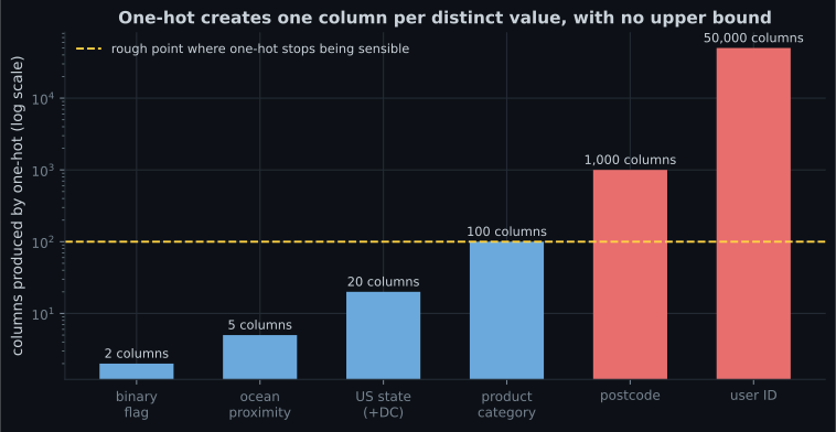
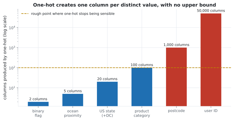
The last row is why sparse matrices exist. A one-hot encoding of a million user IDs is impossible
dense and routine sparse. .toarray() on it will exhaust your memory, which is why scikit-learn
makes you ask.
The dummy variable trap
Section titled “The dummy variable trap”Five one-hot columns always sum to exactly 1, so any one is perfectly predictable from the other four. The design matrix becomes rank-deficient, and for models solved by matrix inversion the solution is not unique.
drop="first" removes one column, making the dropped category the reference level that the
intercept absorbs.
| Model | Does it matter? |
|---|---|
| Linear/logistic regression with an intercept, no regularisation | Yes — drop one |
| Ridge, Lasso, Elastic Net | No — the penalty makes the solution unique anyway |
| Trees, forests, boosting | No — and dropping a column can hurt interpretability |
| Statistical inference (p-values, coefficient CIs) | Yes, always |
scikit-learn’s default is to keep all columns, which is right for regularised and tree-based models — the majority case.
Unseen categories in production
Section titled “Unseen categories in production”Your encoder learned five categories. Six months later a row arrives with "NEAR LAKE".
import pandas as pd
from sklearn.preprocessing import OneHotEncoder

train = pd.DataFrame({"city": ["London", "Paris", "Tokyo"]})
live = pd.DataFrame({"city": ["London", "Berlin"]})       # Berlin is new

strict = OneHotEncoder().fit(train)
try:
    strict.transform(live)
except ValueError as exc:
    print("raised:", str(exc)[:60])
# raised: Found unknown categories ['Berlin'] in column 0 during

safe = OneHotEncoder(handle_unknown="ignore").fit(train)
print(safe.transform(live).toarray())
# [[1. 0. 0.]
#  [0. 0. 0.]]      <- Berlin becomes all zeros
Both behaviours are defensible. Raising catches a data-quality problem loudly; handle_unknown="ignore"
keeps the service running and encodes the unknown as “none of the above”. For anything serving live
traffic, use handle_unknown="ignore" and log the occurrence — an all-zero row is a silent
degradation otherwise.
When one-hot is not an option
Section titled “When one-hot is not an option”| Approach | What it does | Cost |
|---|---|---|
| Frequency encoding | Replace each category with its count or share | Collides: two categories of equal frequency become identical |
| Target encoding | Replace with the mean target for that category | Leaks badly unless cross-fitted and smoothed |
| Hashing | Hash into a fixed number of buckets | Collisions, and no way back to the category |
| Embeddings | Learn a dense vector per category | Needs a neural network and plenty of data |
| Grouping | Keep the top , bucket the rest as “other” | Simple, effective, loses tail detail |
Grouping is the underrated one. Keeping the 20 most common values and folding the remaining 4,980
into other usually captures most of the signal for a fraction of the width.
Pitfalls
Section titled “Pitfalls”-
Why is OrdinalEncoder a poor choice for ocean_proximity with a linear model?
A linear model multiplies the integer code by a coefficient, so the arbitrary alphabetical spacing becomes a real quantitative claim about the categories.
pch.quizShowAnswer
B — It asserts that the categories are ordered and evenly spaced — so the model treats ISLAND as numerically between INLAND and NEAR BAY — A linear model multiplies the integer code by a coefficient, so the arbitrary alphabetical spacing becomes a real quantitative claim about the categories.
-
Why does OneHotEncoder return a sparse matrix by default?
One million rows by 50,000 categories is 400 GB dense and about 12 MB sparse. The default protects you from an allocation that cannot succeed.
pch.quizShowAnswer
B — One-hot output is almost entirely zeros, and storing only the non-zero entries can be thousands of times smaller — One million rows by 50,000 categories is 400 GB dense and about 12 MB sparse. The default protects you from an allocation that cannot succeed.
-
For which model does drop='first' genuinely matter?
The one-hot columns sum to 1, duplicating the intercept. Regularisation makes the solution unique regardless, and trees are unaffected — so scikit-learn keeps every column by default.
pch.quizShowAnswer
B — Unregularised linear regression with an intercept, where the redundant column makes the design matrix rank-deficient — The one-hot columns sum to 1, duplicating the intercept. Regularisation makes the solution unique regardless, and trees are unaffected — so scikit-learn keeps every column by default.
-
A category unseen during training arrives in production. What should a serving pipeline do?
Raising takes the service down; ignoring keeps it up but encodes an uninformative row. Logging turns a silent failure into a signal that the encoder needs refitting.
pch.quizShowAnswer
B — Use handle_unknown='ignore' so the row encodes as all zeros, and log the event so the silent degradation is visible — Raising takes the service down; ignoring keeps it up but encodes an uninformative row. Logging turns a silent failure into a signal that the encoder needs refitting.
🧪 Try It Yourself
Section titled “🧪 Try It Yourself”Exercise 1 – Ordinal-encode and inspect the ordering
Section titled “Exercise 1 – Ordinal-encode and inspect the ordering”Exercise 2 – One-hot encode and read the names
Section titled “Exercise 2 – One-hot encode and read the names”Exercise 3 – Measure the memory saving
Section titled “Exercise 3 – Measure the memory saving”Exercise 4 – Survive an unseen category
Section titled “Exercise 4 – Survive an unseen category”Exercise 5 – Confirm the dummy variable trap
Section titled “Exercise 5 – Confirm the dummy variable trap”- The encoding is a claim about the categories. Ordinal claims an order and a spacing; one-hot claims neither.
OrdinalEncodersorts alphabetically — passcategories=[[...]]whenever the order is real.- Trees can live with ordinal encoding because they split on thresholds; linear models cannot.
- One-hot output is sparse because it must be: a million rows by 50,000 categories is 400 GB dense and 12 MB sparse.
- The one-hot columns sum to 1, so with an unregularised intercept model drop one. Regularised and tree-based models do not care.
- Use
handle_unknown="ignore"in production, and log every occurrence. - Above a few hundred categories, group into a top- plus “other”, or use target encoding done properly with cross-fitting.
Exercise 6 – Measure what each encoding claims
Section titled “Exercise 6 – Measure what each encoding claims”Continue to Feature Scaling (Normalization & Standardization) — every column is numeric now, and they span four orders of magnitude.
pch.coffeeTagline
pch.coffeeCtapch.feedbackHeading
pch.feedbackSubheading