Gradients of Matrices

This is the page where the shapes get away from people.

The rule has not changed — rows are outputs, columns are inputs — but when the input is a matrix, “columns” is no longer one index. Differentiate a matrix with respect to a matrix and you get four indices: two for the output entry, two for the input entry. That is a fourth-order tensor, and the book says so plainly rather than hiding it.

The good news is that there is nothing new to learn, only something to organise. The two ways to organise it are the content of this page, and both appear in the book’s Figure 5.7.

What you’ll learn

• Why $\mathrm{d}f/\mathrm{d}\mathbf{X}$ for matrix arguments is a tensor, and how to read its shape.
• The two ways to make it computable: flatten the matrix into a vector, or partition the tensor into blocks — Figure 5.7’s two panels.
• Example 5.12: $\mathrm{d}(\mathbf{A}\mathbf{x})/\mathrm{d}\mathbf{A}$, and the fact that it is 75% zeros.
• Example 5.13: $\mathrm{d}(\mathbf{R}^\top\mathbf{R})/\mathrm{d}\mathbf{R}$ entry by entry, including the factor of 2 on the diagonal.
• A finding the book does not state: the symmetry of $\mathbf{R}^\top\mathbf{R}$ shows up as a rank deficiency in the flattened Jacobian.
• Why the differential form $\mathrm{d}\mathbf{K} = \mathbf{R}^\top\mathrm{d}\mathbf{R} + \mathrm{d}\mathbf{R}^\top\mathbf{R}$ is the practical way to work, and how it relates to the tensor.

Intuition: four indices, two ways to hold them

Suppose $\mathbf{K} = f(\mathbf{R})$ where $\mathbf{R}$ is $M\times N$ and $\mathbf{K}$ is $N\times N$. The question “how does $\mathbf{K}$ change when $\mathbf{R}$ changes?” needs an answer for every pair of entries: how does $K_{pq}$ respond to $R_{ij}$? That is four indices — $p$, $q$, $i$, $j$ — and $N^2 \cdot MN$ numbers.

You can hold those numbers in two shapes, and the choice is purely one of convenience:

Flatten. Stretch $\mathbf{R}$ into a vector of length $MN$ and $\mathbf{K}$ into one of length $N^2$. Now it is an ordinary Jacobian matrix, $N^2 \times MN$, and every tool from §5.3 applies unchanged. This is what every autodiff library does internally, and it is why a library gradient always comes back with the same shape as the parameter.

Partition. Keep the tensor, but read it as an $N\times N$ grid of $M\times N$ blocks — one block per output entry. Each block is usually a familiar small object, which makes this the version to use by hand.

diagram Diagram mermaid

  flowchart TD
  Q["how does K change when R changes?
K = f(R), R ∈ ℝᴹˣᴺ, K ∈ ℝᴺˣᴺ"]
  Q --> IDX["one number per pair of entries:
∂K_pq / ∂R_ij — FOUR indices"]
  IDX --> T["a fourth-order tensor
ℝ⁽ᴺˣᴺ⁾ˣ⁽ᴹˣᴺ⁾ — Eq 5.94"]
  T --> FLAT["FLATTEN
reshape to an (N²) × (MN) matrix
→ §5.3 applies unchanged
→ what autodiff does internally"]
  T --> PART["PARTITION
an N×N grid of M×N blocks
→ each block is a small familiar object
→ the version to use by hand"]
  T --> DIFF["or avoid it: work with DIFFERENTIALS
dK = RᵀdR + dRᵀR
→ no tensor ever built"]
  FLAT --> SP["and notice the sparsity:
Eq 5.92 is 75% zeros
Eq 5.98 is 44% zeros"]
  DIFF --> ID["§5.5: ten identities that
let you skip the tensor entirely"]

The math

The shape rule, extended

Consider $f:\mathbb{R}^{m\times n}\to\mathbb{R}^{p\times q}$. Then

$$\frac{\mathrm{d}f}{\mathrm{d}\mathbf{X}} \in \mathbb{R}^{(p\times q)\times(m\times n)}$$

a four-dimensional tensor $\mathbf{J}$, whose entries are

$$J_{ijkl} = \frac{\partial f_{ij}}{\partial X_{kl}}$$

The book notes that since matrices represent linear mappings, and since there is a vector-space isomorphism between $\mathbb{R}^{m\times n}$ and $\mathbb{R}^{mn}$, we can re-shape our matrices into vectors of lengths $mn$ and $pq$ respectively. The gradient using these flattened vectors is then a Jacobian of size $pq \times mn$. Figure 5.7 visualises both approaches.

The book’s own practical remark

In practical applications, it is often desirable to re-shape the matrix into a vector and continue working with this Jacobian matrix: The chain rule boils down to simple matrix multiplication, whereas in the case of a Jacobian tensor, we will need to pay more attention to what dimensions we need to sum out.

That is the honest summary. Both organisations are correct; one composes with a @ and the other needs an einsum with the right indices summed.

Example 5.12 — a vector with respect to a matrix

$f = \mathbf{A}\mathbf{x}$ with $f\in\mathbb{R}^M$, $\mathbf{A}\in\mathbb{R}^{M\times N}$, $\mathbf{x}\in\mathbb{R}^N$, and we want $\mathrm{d}f/\mathrm{d}\mathbf{A}$ — the derivative with respect to the matrix this time, not the vector.

Shape first, as always:

$$\frac{\mathrm{d}f}{\mathrm{d}\mathbf{A}} \in \mathbb{R}^{M\times(M\times N)} \tag{5.86}$$

By definition the gradient is the collection of partial derivatives:

$$\frac{\mathrm{d}f}{\mathrm{d}\mathbf{A}} = \begin{bmatrix}\dfrac{\partial f_1}{\partial\mathbf{A}}\\ \vdots\\ \dfrac{\partial f_M}{\partial\mathbf{A}}\end{bmatrix}, \qquad \frac{\partial f_i}{\partial\mathbf{A}} \in \mathbb{R}^{1\times(M\times N)} \tag{5.87}$$

Write out the matrix–vector product explicitly:

$$f_i = \sum_{j=1}^{N}A_{ij}x_j, \qquad i = 1,\dots,M \tag{5.88}$$

and the partial derivatives are

$$\frac{\partial f_i}{\partial A_{iq}} = x_q \tag{5.89}$$

Crucially, $f_i$ depends on row $i$ of $\mathbf{A}$ only. So

$$\frac{\partial f_i}{\partial A_{i,:}} = \mathbf{x}^\top \in \mathbb{R}^{1\times1\times N}, \qquad \frac{\partial f_i}{\partial A_{k\neq i,:}} = \mathbf{0}^\top \in \mathbb{R}^{1\times1\times N} \tag{5.90-5.91}$$

and stacking them,

$$\frac{\partial f_i}{\partial\mathbf{A}} = \begin{bmatrix}\mathbf{0}^\top\\ \vdots\\ \mathbf{0}^\top\\ \mathbf{x}^\top\\ \mathbf{0}^\top\\ \vdots\\ \mathbf{0}^\top\end{bmatrix} \in \mathbb{R}^{1\times(M\times N)} \tag{5.92}$$

with $\mathbf{x}^\top$ in slot $i$ and zeros everywhere else.

Verified for $M = 4$, $N = 3$: the numeric tensor has shape $(4,4,3)$ and matches Equation 5.92 to $1.5\times10^{-10}$. And here is the thing the book does not point out — only 12 of its 48 entries are nonzero, exactly 25%. In general the fraction is $1/M$: each output touches one row.

Example 5.13 — a matrix with respect to a matrix

$\mathbf{R}\in\mathbb{R}^{M\times N}$ and $f:\mathbb{R}^{M\times N}\to\mathbb{R}^{N\times N}$ with

$$f(\mathbf{R}) = \mathbf{R}^\top\mathbf{R} =: \mathbf{K} \in \mathbb{R}^{N\times N} \tag{5.93}$$

The book’s approach to “this hard problem” is to write down what is already known. The shape:

$$\frac{\mathrm{d}\mathbf{K}}{\mathrm{d}\mathbf{R}} \in \mathbb{R}^{(N\times N)\times(M\times N)}, \qquad \frac{\mathrm{d}K_{pq}}{\mathrm{d}\mathbf{R}} \in \mathbb{R}^{1\times M\times N} \tag{5.94-5.95}$$

Then, denoting the $i$-th column of $\mathbf{R}$ by $\mathbf{r}_i$, every entry of $\mathbf{K}$ is an inner product of two columns (§3.2):

$$K_{pq} = \mathbf{r}_p^\top\mathbf{r}_q = \sum_{m=1}^{M}R_{mp}R_{mq} \tag{5.96}$$

Differentiating that sum,

$$\frac{\partial K_{pq}}{\partial R_{ij}} = \sum_{m=1}^{M}\frac{\partial}{\partial R_{ij}}R_{mp}R_{mq} = \partial_{pqij} \tag{5.97}$$ $$\partial_{pqij} = \begin{cases} R_{iq} & \text{if } j = p,\ p \neq q\\ R_{ip} & \text{if } j = q,\ p \neq q\\ 2R_{iq} & \text{if } j = p,\ p = q\\ 0 & \text{otherwise} \end{cases} \tag{5.98}$$

The four cases are the product rule doing its job. $R_{mp}R_{mq}$ is a product of two factors; differentiating with respect to $R_{ij}$ hits the first factor when $j = p$ and the second when $j = q$. When $p = q$ both happen, which is where the $2$ comes from — and that factor of 2 on the diagonal is the single most commonly dropped term in this whole chapter.

Verified for $M = 5$, $N = 3$: the numeric tensor has shape $(3,3,5,3)$, matches Equation 5.98 to $4.8\times10^{-10}$, and the diagonal ratio $\partial K_{pp}/\partial R_{:,p}$ divided by $R_{:,p}$ comes out as exactly $[2, 2, 2, 2, 2]$ for every $p$.

From the book

Section 5.4. The section opens by noting that gradients of matrices with respect to vectors, or matrices with respect to matrices, give multidimensional tensors, and that since matrices represent linear mappings and $\mathbb{R}^{m\times n}$ is isomorphic to $\mathbb{R}^{mn}$, the matrices can be re-shaped into vectors so the gradient becomes an ordinary Jacobian of size $pq\times mn$. Figure 5.7 draws both views for $\mathbf{A}\in\mathbb{R}^{4\times2}$ with respect to $\mathbf{x}\in\mathbb{R}^3$: three $4\times2$ matrices collated into a $4\times2\times3$ tensor, or an $8\times3$ Jacobian matrix. A Remark recommends the re-shaped version in practice, because the chain rule then reduces to matrix multiplication rather than requiring care about which dimensions to sum out. Example 5.12 (Equations 5.85 to 5.92) computes $\mathrm{d}(\mathbf{A}\mathbf{x})/\mathrm{d}\mathbf{A}$, using the fact that $f_i$ depends only on row $i$. Example 5.13 (Equations 5.93 to 5.98) computes $\mathrm{d}(\mathbf{R}^\top\mathbf{R})/\mathrm{d}\mathbf{R}$ entry by entry, with the four-case formula of Equation 5.98.

Worked example by hand

Equation 5.98’s four cases, on a 2 by 2

Take $M = N = 2$, so $\mathbf{R} = \begin{bmatrix}a&b\\c&d\end{bmatrix}$ and

$$\mathbf{K} = \mathbf{R}^\top\mathbf{R} = \begin{bmatrix}a^2+c^2 & ab+cd\\ ab+cd & b^2+d^2\end{bmatrix}$$

Now differentiate each entry with respect to each entry of $\mathbf{R}$, and check against Equation 5.98:

$K_{pq}$	$\partial/\partial a$	$\partial/\partial b$	$\partial/\partial c$	$\partial/\partial d$	which case of 5.98
$K_{11} = a^2+c^2$	$2a$	$0$	$2c$	$0$	$p=q=1$: $2R_{i1}$ when $j=1$, else $0$
$K_{12} = ab+cd$	$b$	$a$	$d$	$c$	$p=1,q=2$: $R_{i2}$ when $j=1$; $R_{i1}$ when $j=2$
$K_{21} = ab+cd$	$b$	$a$	$d$	$c$	same, by symmetry
$K_{22} = b^2+d^2$	$0$	$2b$	$0$	$2d$	$p=q=2$: $2R_{i2}$ when $j=2$, else $0$

Read the first row: differentiating $a^2 + c^2$ with respect to $a$ gives $2a$, and Equation 5.98’s third case with $p=q=1$, $i=1$, $j=1$ gives $2R_{11} = 2a$. ✓

Read the second row: $\partial(ab+cd)/\partial a = b$, and the first case with $p=1$, $q=2$, $i=1$, $j=1$ gives $R_{12} = b$. ✓

The rows for $K_{12}$ and $K_{21}$ are identical, which they must be because $\mathbf{K}$ is symmetric. Measured on a $5\times3$: the worst asymmetry $\lVert\partial K_{pq}/\partial\mathbf{R} - \partial K_{qp}/\partial\mathbf{R}\rVert$ is exactly 0.0e+00.

A finding: the symmetry becomes a rank deficiency

Flatten that tensor for $M=5$, $N=3$ and you get a $9\times15$ matrix. Its rank is not $9$:

$$\mathrm{rank}\left(\text{flattened } \frac{\mathrm{d}\mathbf{K}}{\mathrm{d}\mathbf{R}}\right) = 6 = \frac{N(N+1)}{2}$$

Because $\mathbf{K}$ is symmetric, only $6$ of its $9$ entries are independent — and the Jacobian knows. Three of its rows are exact duplicates of three others, so the flattened Jacobian has a three-dimensional left null space.

This matters in practice. If you feed such a Jacobian to a solver expecting full rank, it will be singular, and the reason is not numerical: it is that you asked for the derivative of nine quantities of which only six are free. Working with $\mathbf{K}$‘s upper triangle instead gives a $6\times15$ Jacobian of full rank $6$.

The differential form: how to avoid the tensor entirely

There is a third option, and it is what people actually do. Instead of building the tensor, perturb and read off:

$$\mathbf{K} + \mathrm{d}\mathbf{K} = (\mathbf{R}+\mathrm{d}\mathbf{R})^\top(\mathbf{R}+\mathrm{d}\mathbf{R}) = \mathbf{R}^\top\mathbf{R} + \mathbf{R}^\top\mathrm{d}\mathbf{R} + \mathrm{d}\mathbf{R}^\top\mathbf{R} + O(\mathrm{d}\mathbf{R}^2)$$

so

$$\boxed{\;\mathrm{d}\mathbf{K} = \mathbf{R}^\top\mathrm{d}\mathbf{R} + \mathrm{d}\mathbf{R}^\top\mathbf{R}\;}$$

No four-index object appears. Verified: for a random direction $\mathbf{H}$ the central difference $\bigl[(\mathbf{R}+h\mathbf{H})^\top(\mathbf{R}+h\mathbf{H}) - (\mathbf{R}-h\mathbf{H})^\top(\mathbf{R}-h\mathbf{H})\bigr]/2h$ agrees with $\mathbf{R}^\top\mathbf{H} + \mathbf{H}^\top\mathbf{R}$ to $8.5\times10^{-10}$, and contracting the full tensor against $\mathbf{H}$ with einsum("pqij,ij->pq", T, H) gives the same to $3.6\times10^{-10}$.

The differential form and the tensor are the same information. The differential is a directional statement, and contracting the tensor with a direction is how you recover it. §5.5’s ten identities are all differentials, which is why they are usable by hand.

See it move

sketch Four indices, two shapes p5.js Pause Restart

The same tensor, drawn both ways. Left: an N-by-N grid of M-by-N blocks, one block per output entry — the partitioned view. Right: the flattened Jacobian matrix. Scrub the output entry (p,q) and watch which block lights up and which row of the matrix it corresponds to. The numbers are Equation 5.98's, for a matrix you can edit.

sketch Example 5.12 is mostly zeros p5.js Pause Restart

The tensor df/dA for f = Ax, drawn as M slices of M-by-N. Only one row of each slice is nonzero, because output i depends on row i of A alone. Drag M and N and watch the sparsity — the nonzero fraction is exactly 1/M, whatever the shape.

From scratch

matrix_gradients_from_scratch.py

import numpy as np
 
def tensor_jac(f, X, h=1e-6):
    """Full Jacobian tensor: shape f(X).shape + X.shape, by central differences."""
    X = np.asarray(X, dtype=float)
    F0 = np.asarray(f(X))
    J = np.zeros(F0.shape + X.shape)
    it = np.nditer(X, flags=["multi_index"])
    while not it.finished:
        idx = it.multi_index
        Xp = X.copy(); Xp[idx] += h
        Xm = X.copy(); Xm[idx] -= h
        J[(Ellipsis,) + idx] = (np.asarray(f(Xp)) - np.asarray(f(Xm))) / (2 * h)
        it.iternext()
    return J
 
rng = np.random.default_rng(5)
 
# ---- Figure 5.7: dA/dx where A in R^{4x2} depends on x in R^3
B = rng.normal(size=(4, 2, 3))
x0 = rng.normal(size=3)
T = tensor_jac(lambda x: B @ x, x0)
print("Figure 5.7")
print(f"  dA/dx tensor shape    {T.shape}   (the book's 4 x 2 x 3)")
print(f"  flattened             {T.reshape(4*2, 3).shape}   = (mn) x p, the other panel")
print(f"  same numbers?         {np.allclose(T.reshape(4*2, 3).reshape(T.shape), T)}")
 
# ---- Example 5.12: f = Ax, df/dA
M, N = 4, 3
A = rng.normal(size=(M, N))
x = rng.normal(size=N)
T = tensor_jac(lambda Am: Am @ x, A)
pred = np.zeros((M, M, N))
for i in range(M):
    pred[i, i, :] = x                                  # Eq 5.92
print()
print("Example 5.12")
print(f"  df/dA shape           {T.shape}   -- Eq 5.86 predicted {M} x ({M} x {N})")
print(f"  matches Eq 5.92 to    {np.abs(T - pred).max():.1e}")
print(f"  nonzero entries       {int(np.sum(np.abs(T) > 1e-9))} of {T.size}"
      f"  ({100*np.sum(np.abs(T) > 1e-9)/T.size:.1f}%  =  1/M)")
 
# ---- Example 5.13: f(R) = R^T R
Mr, Nr = 5, 3
R = rng.normal(size=(Mr, Nr))
T = tensor_jac(lambda Rm: Rm.T @ Rm, R)
 
def eq_5_98(R, p, q, i, j):
    if j == p and p != q:
        return R[i, q]
    if j == q and p != q:
        return R[i, p]
    if j == p and p == q:
        return 2 * R[i, q]
    return 0.0
 
pred = np.zeros_like(T)
for p in range(Nr):
    for q in range(Nr):
        for i in range(Mr):
            for j in range(Nr):
                pred[p, q, i, j] = eq_5_98(R, p, q, i, j)
 
print()
print("Example 5.13")
print(f"  dK/dR shape           {T.shape}   -- Eq 5.94 predicted ({Nr}x{Nr}) x ({Mr}x{Nr})")
print(f"  matches Eq 5.98 to    {np.abs(T - pred).max():.1e}")
print(f"  nonzero entries       {int(np.sum(np.abs(T) > 1e-9))} of {T.size}"
      f"  ({100*np.sum(np.abs(T) > 1e-9)/T.size:.1f}%)")
sym = max(float(np.abs(T[p, q] - T[q, p]).max()) for p in range(Nr) for q in range(Nr))
print(f"  worst asymmetry       {sym:.1e}  (K is symmetric, so this must vanish)")
for p in range(Nr):
    ratio = T[p, p, :, p] / R[:, p]
    print(f"  dK{p}{p}/dR[:,{p}] / R[:,{p}] = {np.round(ratio, 6)}   <- Eq 5.98's factor of 2")
 
# ---- the rank deficiency the symmetry causes
flatJ = T.reshape(Nr * Nr, Mr * Nr)
print()
print("Flattened, and the consequence of symmetry")
print(f"  as a matrix           {flatJ.shape} = (N*N) x (M*N)")
print(f"  rank                  {np.linalg.matrix_rank(flatJ)} of {min(flatJ.shape)}")
print(f"  N(N+1)/2              {Nr*(Nr+1)//2}   <- the number of FREE entries of K")
 
# ---- and the differential form, which never builds a tensor
H = rng.normal(size=(Mr, Nr))
h = 1e-6
num = ((R + h*H).T @ (R + h*H) - (R - h*H).T @ (R - h*H)) / (2*h)
ana = R.T @ H + H.T @ R
print()
print("The differential form dK = R^T dR + dR^T R")
print(f"  vs a central difference        {np.abs(num - ana).max():.1e}")
print(f"  vs contracting the tensor      "
      f"{np.abs(np.einsum('pqij,ij->pq', T, H) - ana).max():.1e}")

output

Figure 5.7
  dA/dx tensor shape    (4, 2, 3)   (the book's 4 x 2 x 3)
  flattened             (8, 3)   = (mn) x p, the other panel
  same numbers?         True
 
Example 5.12
  df/dA shape           (4, 4, 3)   -- Eq 5.86 predicted 4 x (4 x 3)
  matches Eq 5.92 to    1.5e-10
  nonzero entries       12 of 48  (25.0%  =  1/M)
 
Example 5.13
  dK/dR shape           (3, 3, 5, 3)   -- Eq 5.94 predicted (3x3) x (5x3)
  matches Eq 5.98 to    4.8e-10
  nonzero entries       75 of 135  (55.6%)
  worst asymmetry       0.0e+00  (K is symmetric, so this must vanish)
  dK00/dR[:,0] / R[:,0] = [2. 2. 2. 2. 2.]   <- Eq 5.98's factor of 2
  dK11/dR[:,1] / R[:,1] = [2. 2. 2. 2. 2.]   <- Eq 5.98's factor of 2
  dK22/dR[:,2] / R[:,2] = [2. 2. 2. 2. 2.]   <- Eq 5.98's factor of 2
 
Flattened, and the consequence of symmetry
  as a matrix           (9, 15) = (N*N) x (M*N)
  rank                  6 of 9
  N(N+1)/2              6   <- the number of FREE entries of K
 
The differential form dK = R^T dR + dR^T R
  vs a central difference        8.5e-10
  vs contracting the tensor      3.6e-10

Four readings.

The two panels of Figure 5.7 are the same numbers. reshape is free and reversible, which is why “flatten it” is sound advice rather than a lossy shortcut.

Example 5.12 is 75% zeros, and the fraction is exactly $1/M$ regardless of $N$. The book derives that structure at Equations 5.90–5.91 without naming its consequence: a naive dense tensor wastes a factor of $M$ in memory. For a linear layer with $M = 1024$ outputs that is a factor of a thousand, which is why no framework ever materialises this object.

The asymmetry is exactly 0.0e+00. $K_{pq}$ and $K_{qp}$ are literally the same sum, so their derivatives are computed from the same floating-point operations and agree bit-for-bit. That is a check on the construction; the mathematical content is that the tensor inherits every symmetry the function has.

And the rank is 6, not 9. The symmetry that showed up as duplicate slices shows up in the flattened matrix as a rank deficiency of exactly $N^2 - N(N+1)/2 = 3$.

On real data

figure The shape bookkeeping of §5.4 matplotlib

Five functions, from a scalar of a matrix up to a matrix of a matrix. The shape column is the whole point: a scalar of an E-by-F matrix gives 1 x (E x F), while a matrix of a matrix gives a fourth-order tensor. Underneath, the two ways to make that computable.

figure Eight identities, each checked numerically matplotlib

Every rule §5.4 and §5.5 rely on, differenced independently. The worst disagreement is 6.1e-10, for the determinant rule — which is the level a central difference at h = 1e-6 can reach, so the bars measure the test's floor rather than the identities' error.

figure d tr(AXB) / dX = (BA)-transpose, drawn matplotlib

A is 2x7 and B is 6x2, so BA has rank at most 2 — and the measured rank of the 7x6 gradient is exactly 2. The gradient of a scalar function of a matrix always has the SHAPE of that matrix, and here it inherits a rank ceiling from the factors too.

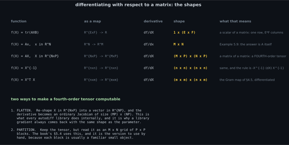
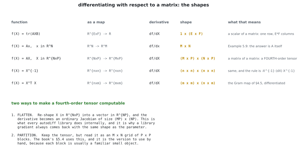
Reading the plot

From the shape ladder. Read the shape column downwards and the escalation is clear: a scalar of a vector is a row, a vector of a vector is a matrix, a matrix of a matrix is a tensor. Nothing about the rule changed — it is always $\partial(\text{output index})/\partial(\text{input index})$ — only the number of indices.

The two strategies at the bottom are not equivalent in practice. Flattening makes the chain rule a @; partitioning keeps the structure visible. If you are deriving on paper, partition. If you are writing code, flatten — and if you are using a framework, it has already flattened for you, which is why param.grad always has param.shape.

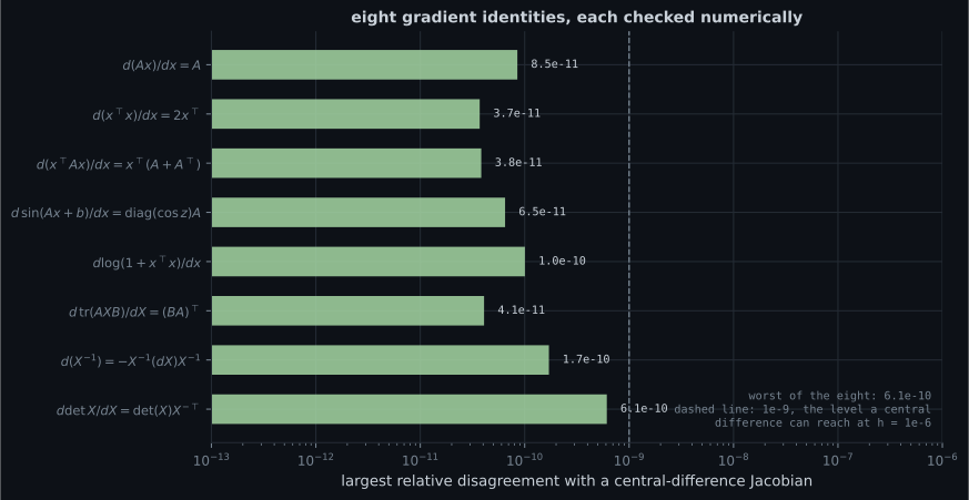
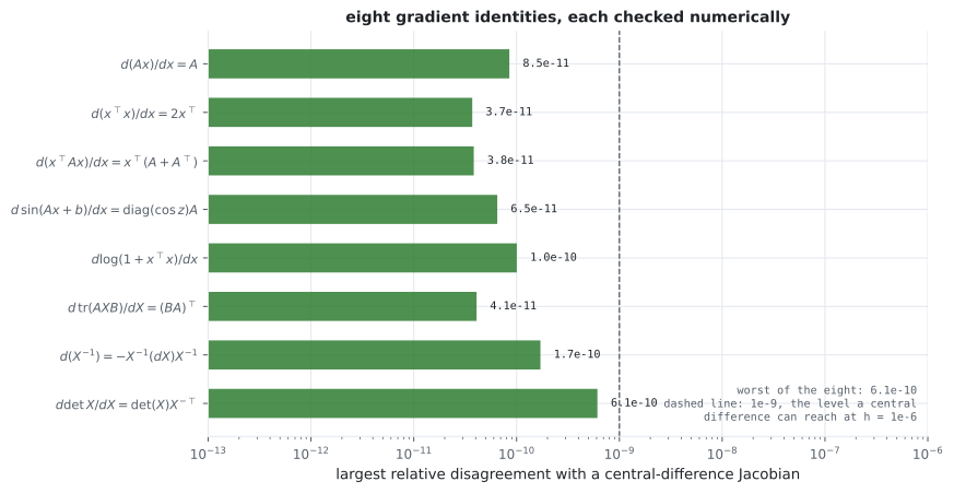
From the identities figure. Eight rules, eight bars, all between $3.7\times10^{-11}$ and $6.1\times10^{-10}$. The important thing about that range is that it is the test’s floor, not the identities’ error: a central difference at $h = 10^{-6}$ cannot do better than about $10^{-10}$ relative, as §5.1’s figure showed. So these bars say “consistent with exact”, and a rule with a transposed factor would sit at $10^{0}$, not $10^{-9}$.

The worst bar is $\mathrm{d}\det\mathbf{X}/\mathrm{d}\mathbf{X}$ at $6.1\times10^{-10}$, which is unsurprising: the determinant of a $3\times3$ amplifies input perturbations by roughly its own condition number, so the difference quotient has further to fall.

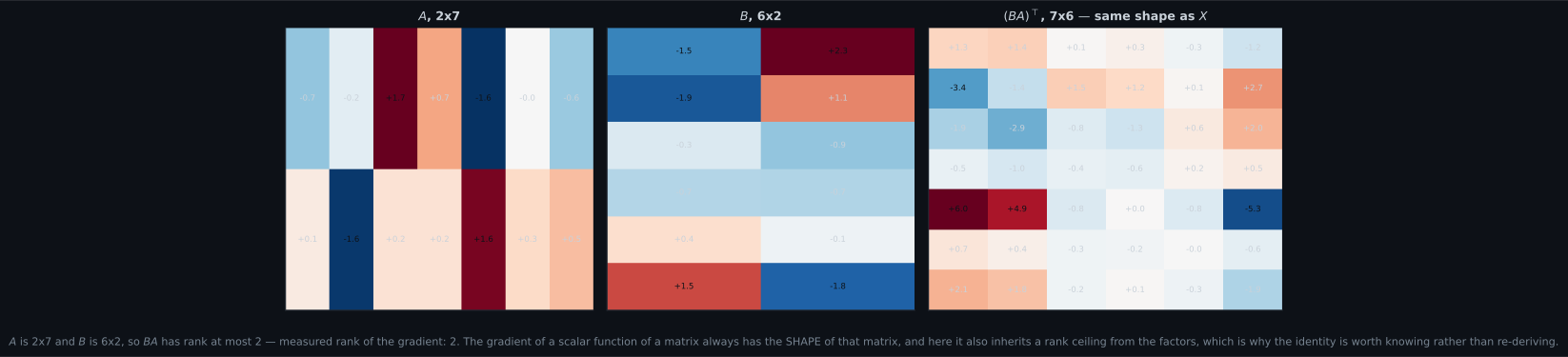
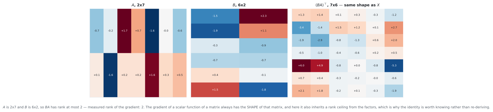
From the trace figure. Two facts in one picture. The gradient has the shape of $\mathbf{X}$ — $7\times6$, not $1\times42$ — which is what makes $\mathrm{d}\,\mathrm{tr}(\mathbf{A}\mathbf{X}\mathbf{B})/\mathrm{d}\mathbf{X} = (\mathbf{B}\mathbf{A})^\top$ usable directly as an update. And its rank is capped by the inner dimension: $\mathbf{A}$ is $2\times7$ and $\mathbf{B}$ is $6\times2$, so $\mathbf{B}\mathbf{A}$ factors through $\mathbb{R}^2$ and cannot have rank above $2$. Measured: exactly $2$.

That rank ceiling is why low-rank adapters work. If a loss depends on $\mathbf{X}$ only through $\mathbf{A}\mathbf{X}\mathbf{B}$ with thin $\mathbf{A}$ and $\mathbf{B}$, then every gradient it will ever produce lies in a rank-2 subspace — so there is no point storing a full-rank update.

Pitfalls

The factor of 2 on the diagonal of Equation 5.98

When $p = q$ both product-rule terms fire on the same entry, giving $2R_{iq}$. It is the single most commonly dropped term in this chapter, and it is dropped silently: the off-diagonal entries are still right, so the result looks plausible. Measured check that catches it: $\partial K_{pp}/\partial R_{:,p}$ divided by $R_{:,p}$ must be exactly $2$, which it is — $[2,2,2,2,2]$ for every $p$.

A flattened Jacobian of a symmetric output is rank-deficient by construction

$\mathrm{d}(\mathbf{R}^\top\mathbf{R})/\mathrm{d}\mathbf{R}$ flattens to a $9\times15$ matrix of rank $6$, not $9$, because only $N(N+1)/2$ entries of a symmetric $N\times N$ matrix are free. Hand that to a solver expecting full rank and it will be singular — and the cause is not numerical conditioning, it is that you asked for the derivative of nine quantities of which three are copies. Differentiate the upper triangle instead.

Never materialise the dense tensor

Example 5.12’s tensor is $1/M$ dense. At $M = 1024$ that is a factor of a thousand wasted, and the tensor itself is $M^2N$ numbers — for a $1024\times1024$ layer, $10^9$ entries to hold an object whose content is one vector $\mathbf{x}$. Frameworks store the contraction you actually need, never the tensor.

einsum needs the right indices summed; a matrix product does not

The book’s remark is the practical warning: after flattening, the chain rule is matrix multiplication and the shapes check themselves. Keep the tensor and you need einsum("pqij,ij->pq", T, H) — and einsum("pqij,ij->qp", T, H) runs perfectly well while computing the transpose of what you wanted. There is no shape error to catch it.

Differentials are usually the right tool by hand

$\mathrm{d}\mathbf{K} = \mathbf{R}^\top\mathrm{d}\mathbf{R} + \mathrm{d}\mathbf{R}^\top\mathbf{R}$ takes two lines and never mentions four indices. It is a directional statement, and contracting the full tensor with a direction recovers it — verified here to $3.6\times10^{-10}$. §5.5’s ten identities are all in this form, which is why they are usable.

Compare

you want	the object	shape	how to get it
$\partial(\text{scalar})/\partial\text{vector}$	gradient	$1\times n$	§5.2, Equation 5.40
$\partial\text{vector}/\partial\text{vector}$	Jacobian	$m\times n$	§5.3, Definition 5.6
$\partial(\text{scalar})/\partial\text{matrix}$	gradient	$1\times(E\times F)$, or reshaped to $E\times F$	§5.5’s identities
$\partial\text{vector}/\partial\text{matrix}$	3-tensor	$M\times(M\times N)$	Example 5.12
$\partial\text{matrix}/\partial\text{matrix}$	4-tensor	$(p\times q)\times(m\times n)$	Example 5.13
the derivative in one direction	a matrix	the shape of the output	a differential — usually what you want
the derivative for code	a flattened Jacobian	$pq\times mn$	reshape, then §5.3

pch.quizTag Check your understanding

1. Why does differentiating a matrix with respect to a matrix give a fourth-order tensor?

   A Because matrices are two-dimensional B Because the rule is unchanged — one number per (output index, input index) pair — and each index is now itself a pair, so there are four indices in total C Because the chain rule needs four factors D Because the derivative of a matrix is a matrix of matrices
   pch.quizShowAnswer

   B — Because the rule is unchanged — one number per (output index, input index) pair — and each index is now itself a pair, so there are four indices in total — Nothing new is being defined. Definition 5.6's rule still holds; it is just that 'the output index' and 'the input index' each split into two when the objects are matrices.

2. The book recommends re-shaping matrices into vectors. What does that buy, and what does it cost?

   A It is purely cosmetic B It makes the chain rule a plain matrix multiplication whose shapes check themselves; the cost is that the block structure stops being visible, so it is worse for deriving by hand C It reduces the number of entries D It makes the gradient exact
   pch.quizShowAnswer

   B — It makes the chain rule a plain matrix multiplication whose shapes check themselves; the cost is that the block structure stops being visible, so it is worse for deriving by hand — The book's remark says exactly this: with a tensor you must pay attention to which dimensions to sum out. And einsum with the wrong output index order runs fine while computing a transpose — there is no shape error to catch it.

3. Example 5.12's tensor is 25 percent nonzero for M = 4. Where does that fraction come from?

   A The particular x chosen B From Equations 5.90 and 5.91: output f-i depends on row i of A alone, so each of the M slices has one nonzero row out of M. The fraction is exactly 1/M, whatever N is C From the sparsity of A D From the finite-difference tolerance
   pch.quizShowAnswer

   B — From Equations 5.90 and 5.91: output f-i depends on row i of A alone, so each of the M slices has one nonzero row out of M. The fraction is exactly 1/M, whatever N is — At M = 1024 that is a factor of a thousand wasted if you materialise the tensor. Frameworks store the contraction you need instead — this object is never built.

4. Flattening dK/dR for K = R-transpose R gives a 9 by 15 matrix of rank 6, not 9. Why?

   A Numerical conditioning B Because K is symmetric, so only N(N+1)/2 = 6 of its 9 entries are independent — three rows of the Jacobian are exact duplicates of three others. The deficiency is structural, not numerical C Because R is 5 by 3 and 15 > 9 D Because the finite differences lost rank
   pch.quizShowAnswer

   B — Because K is symmetric, so only N(N+1)/2 = 6 of its 9 entries are independent — three rows of the Jacobian are exact duplicates of three others. The deficiency is structural, not numerical — The same fact appears in the tensor as slices that are exactly equal: the measured asymmetry between dKpq/dR and dKqp/dR is 0.0e+00. Differentiate the upper triangle and you get a full-rank 6 by 15 Jacobian.

5. What is the practical alternative to building the tensor at all?

   A Use finite differences B Work with differentials: perturbing K = R-transpose R gives dK = R-transpose dR + dR-transpose R in two lines, with no four-index object. Contracting the full tensor with a direction recovers exactly this C Assume the tensor is sparse D Flatten to a vector and use §5.2
   pch.quizShowAnswer

   B — Work with differentials: perturbing K = R-transpose R gives dK = R-transpose dR + dR-transpose R in two lines, with no four-index object. Contracting the full tensor with a direction recovers exactly this — Verified to 3.6e-10 against the contracted tensor and 8.5e-10 against a central difference. All ten identities in §5.5 are differentials, which is precisely why they are usable by hand.

🧪 Try It Yourself

Exercise 1 – Figure 5.7, both panels

pch.exerciseTag pch.exerciseTitle

Exercise 2 – Example 5.12, and its sparsity

pch.exerciseTag pch.exerciseTitle

Exercise 3 – Equation 5.98, entry by entry

pch.exerciseTag pch.exerciseTitle

Exercise 4 – The symmetry becomes a rank deficiency

pch.exerciseTag pch.exerciseTitle

Exercise 5 – Differentials, and the einsum trap

pch.exerciseTag pch.exerciseTitle

Recall card

• The shape rule never changes — one number per (output index, input index) pair — but a matrix argument makes each index a pair, so a matrix of a matrix is a fourth-order tensor of shape (p×q)×(m×n).
• Two ways to organise it. Flatten to a (pq)×(mn) Jacobian so the chain rule is a matrix product; or partition into a grid of blocks, which keeps the structure visible for hand work. Figure 5.7 shows both, and they hold identical numbers.
• The book’s own advice is to flatten in practice, because with a tensor you must attend to which dimensions to sum out.
• Example 5.12: df/dA for f = Ax has x-transpose in slot i and zeros elsewhere, because output i touches row i alone. Measured nonzero fraction exactly 1/M — 25% at M = 4, 20% at M = 5.
• Example 5.13: every entry of dK/dR for K = R-transpose R is Equation 5.98’s four-case formula, verified to 4.8e-10 across all 135 entries.
• The factor of 2 appears when p = q, because both product-rule terms fire on the same entry. The measured diagonal ratio is exactly 2 at every entry, and dropping it leaves the off-diagonals right — so the mistake looks plausible.
• K is symmetric, so dKpq/dR and dKqp/dR are bit-for-bit identical (asymmetry 0.0e+00), and the flattened Jacobian is rank-deficient by exactly N² − N(N+1)/2. Differentiate the upper triangle to get full rank.
• Differentials avoid the tensor entirely: dK = R-transpose dR + dR-transpose R, two lines, no four-index object. Contracting the tensor with a direction recovers it to 3.6e-10.
• einsum has no shape check for a transposed output index. pqij,ij->qp runs fine and computes the transpose; on a symmetric output it even gives the right answer, so the bug hides.
• Never materialise the dense tensor. Example 5.12’s is M²N numbers to hold the content of one vector.

Next: Useful Identities for Computing Gradients — ten differentials that let you skip all of this.