Capstone 1 - An Image Classifier End to End

This capstone is the whole module applied to one problem: Fashion-MNIST, ten garment classes, 12,000 training images and 3,000 held out. Not MNIST — MNIST is easy enough that a linear model reaches 0.92 and every later rung has nothing left to show.

The deliverable is not a model. It is a ladder of models, each one measured against the rung below it, ending in something small enough to ship:

Model	Parameters	Accuracy	Gain over the rung below
Always predict one class	0	0.0993	—
Nearest class centroid	7,840	0.6713	+0.5720
Linear (softmax)	7,850	0.8290	+0.1577
MLP	109,386	0.8603	+0.0313
Convnet	225,034	0.8773	+0.0170
Convnet + augmentation	225,034	0.8643	−0.0130

Read the gain column. Each rung buys less than the one before, and the last one is negative — augmentation made the held-out score worse. That looks like a failed experiment. It is the most useful result on the page, and the rest of it explains why.

What you’ll learn

• How to build a baseline ladder, and why the gaps matter more than the final number.
• Why a technique that lowers your test score can still be the right choice.
• How to take the chosen model through pruning and conversion, measuring at each step.
• What to report when you hand this in.

The ladder

figure 3,000 held-out garments, identical split at every rung matplotlib

The first two rungs do most of the work: a nearest-centroid classifier with no gradient descent at all reaches 0.6713, and a linear model reaches 0.8290. Everything after that — a 14x increase in parameters and a 16x increase in training time — buys a combined 0.0483. That ratio is what a baseline ladder is for, and it is invisible if you only ever train the last model.

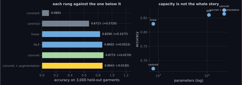
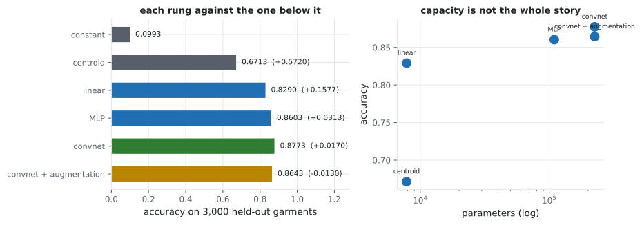
Start at the bottom, always. The constant predictor tells you the class balance (0.0993 here, so the classes are even). The centroid classifier tells you how much of the problem is solved by “which class does this look most like on average” — 0.6713, which is two thirds of it.

The linear model at 0.8290 is the number that should discipline everything after it. It has 7,850 parameters and trains in four seconds. The convnet has 28× more parameters, takes 16× longer and adds 0.0483. On a real project that trade might well be the wrong one, and you cannot know without having built both.

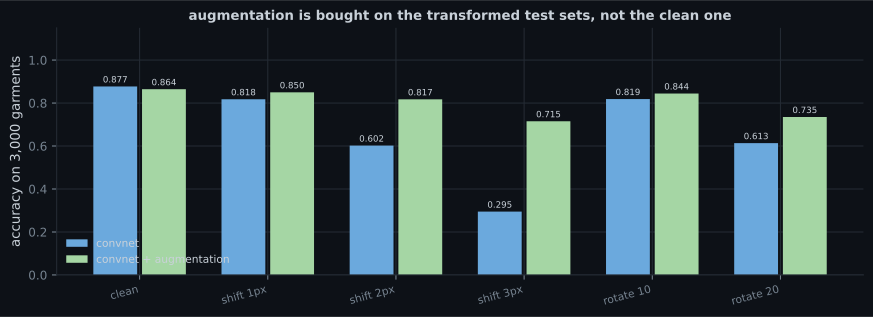
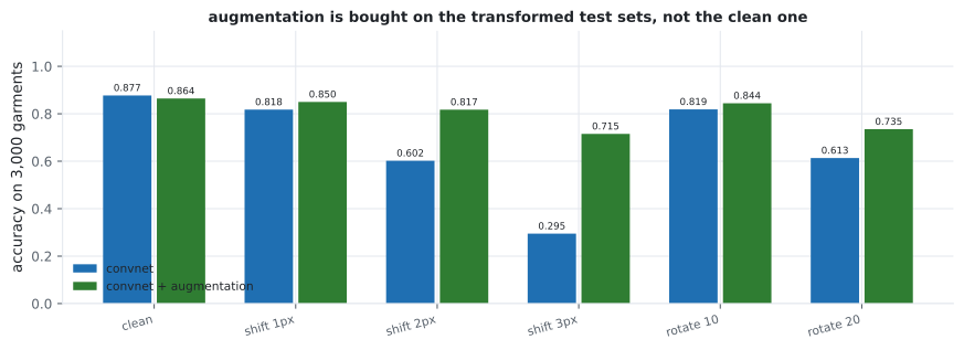
The result that looks like a failure

The convnet reached 0.8974 on its training set against 0.8773 held out. That 0.0201 gap is what augmentation exists to close — and when applied, it lowered the held-out score to 0.8643.

Reported on the clean test set alone, augmentation is a regression. So test it on something else:

figure The same two models, six versions of the test set matplotlib

The clean column is the only one where the plain convnet wins, and it wins by 0.0130. On a three-pixel shift — a change no human would remark on — the plain model collapses to 0.2947 while the augmented one holds 0.7153, a gap of 0.4207. Augmentation did not cost accuracy; it moved accuracy from a distribution you will not deploy on to distributions you might.

Test set	Convnet	Augmented	Delta
Clean	0.8773	0.8643	−0.0130
Shift 1 px	0.8177	0.8500	+0.0323
Shift 2 px	0.6020	0.8173	+0.2153
Shift 3 px	0.2947	0.7153	+0.4207
Rotate 10°	0.8187	0.8443	+0.0257
Rotate 20°	0.6133	0.7350	+0.1217

This is the capstone’s central lesson, and it generalises well past augmentation: a single test number cannot tell you whether a change was good. The plain convnet is better on the distribution it was measured on and dramatically worse everywhere near it. Which model you want depends on whether your deployed inputs will be perfectly centred — and they will not be.

The cost is real too: 24 epochs against 12, and 189 seconds against 66, because augmented data is harder to fit and needs longer to converge. A run that gave augmentation the same 12-epoch budget would have measured its cost and none of its benefit.

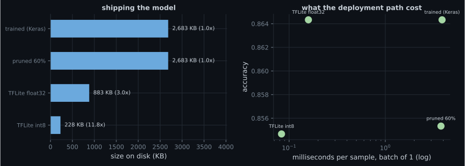
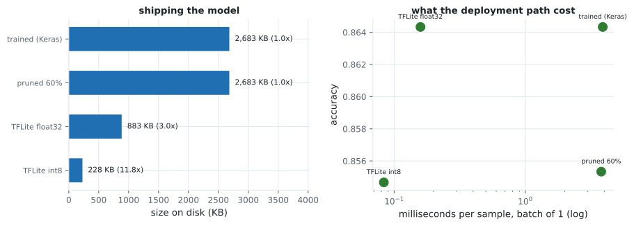
Shipping it

The augmented convnet is the model to deploy. Here is what the deployment path did to it:

figure One model, four artefacts matplotlib

The pruned bar is the instructive one: 60% of the weight matrices are zero and the file is 0.3 KB smaller, because a .keras file stores zeros like any other float. The size win comes entirely from conversion and quantisation — 11.8x — and the latency win of 47x comes from leaving the Keras runtime, not from making the model smaller.

Artefact	Size	Accuracy	ms/sample
Trained (Keras)	2,683.1 KB	0.8643	3.893
Pruned 60%	2,682.8 KB	0.8553	3.792
TFLite float32	883.4 KB	0.8643	0.159
TFLite int8	228.2 KB	0.8547	0.083

Pruning to 60% dropped accuracy to 0.8067 immediately and recovered to 0.8553 after three epochs of fine-tuning with the mask re-applied each epoch. That recovery step is the technique; without it the number to report would have been 0.8067.

The final artefact is 11.8× smaller and 47× faster per sample for 0.0096 of accuracy.

diagram Diagram mermaid

  flowchart LR
  B["constant 0.0993"] --> C["centroid 0.6713"]
  C --> L["linear 0.8290"]
  L --> M["MLP 0.8603"]
  M --> V["convnet 0.8773"]
  V --> A["augmented 0.8643"]
  A --> P["pruned 60% 0.8553"]
  P --> T["TFLite int8 0.8547
228 KB, 0.083 ms"]
  V -.->|"clean test only"| X["looks best"]
  A -.->|"shifted 3px: 0.7153 vs 0.2947"| Y["actually best"]

What to hand in

A defensible submission for this project is short and contains no adjectives:

1. The ladder, including the rungs that did not help. The negative gain from augmentation is part of the result.
2. At least one off-distribution evaluation. Clean accuracy alone would have chosen the wrong model here.
3. The training/held-out gap for the chosen model, so overfitting is visible rather than inferred.
4. The deployment table: size, accuracy and latency at each step, with the immediate post-pruning number as well as the recovered one.
5. The budget. 12 epochs, 24 for the augmented run, on 12,000 images on a CPU — every number above is conditional on that.

sketch Which model wins depends on the test set p5.js Pause Restart

Click a test condition. The bars are the two convnets measured on that version of the test set, and the verdict changes with the condition.

sketch The measured table, ranked p5.js Pause Restart

Click a column to rank every row by it. The bars are that column's values and the highest and lowest are computed from the numbers, not written in.

Pitfalls

• Skipping the baselines. A centroid classifier reached 0.6713 here; without it, 0.8773 sounds like the model did all the work.
• Judging augmentation on clean data. It lost 0.0130 there and won 0.4207 three pixels away.
• Giving augmentation the same epoch budget. Augmented data is harder to fit; 12 epochs would have shown the cost and hidden the benefit.
• Reporting the pruned model without fine-tuning. 0.8067 against 0.8553.
• Expecting a pruned .keras file to be smaller. It was 0.3 KB smaller at 60% sparsity.
• Measuring latency through Keras. 3.893 ms against 0.083 ms for the same computation in TFLite at batch 1.
• Reading the last rung as the only result. The interesting numbers here are the gaps between rungs, not the top of the ladder.

Recap

• The ladder ran 0.0993 → 0.6713 → 0.8290 → 0.8603 → 0.8773, with each rung buying less than the one before.
• A linear model with 7,850 parameters got within 0.0483 of a convnet with 225,034.
• Augmentation cost 0.0130 on clean data and gained 0.4207 on a three-pixel shift.
• The convnet’s 0.0201 train/test gap is what augmentation was brought in to close.
• Pruning 60% needed fine-tuning to go from 0.8067 back to 0.8553, and saved no disk space.
• The deployed artefact is 11.8× smaller and 47× faster for 0.0096 of accuracy.

Next

The same ladder, applied to text — where it stops climbing much earlier: Capstone 2 - A Text Classifier End to End.

pch.quizTag pch.quizDefaultTitle

1. Augmentation lowered clean test accuracy from 0.8773 to 0.8643 but raised three-pixel-shift accuracy from 0.2947 to 0.7153. Which model should be deployed?

   A The plain convnet, since it scores higher on the test set B The augmented one, unless you are certain deployed inputs will be as perfectly centred as the test set — a single test number cannot decide this C Neither; retrain until clean accuracy improves D It makes no difference
   pch.quizShowAnswer

   B — The augmented one, unless you are certain deployed inputs will be as perfectly centred as the test set — a single test number cannot decide this — The clean test set is one distribution. The measurement that matters is performance on the distribution you will actually see, which is why the off-distribution evaluation is part of the deliverable.

2. A nearest-centroid classifier with no gradient descent reached 0.6713 and a linear model 0.8290, while a convnet reached 0.8773. What does the ladder tell you?

   A The convnet is 0.8773 accurate, which is what matters B Most of the problem is solved by very simple methods — the convnet's 28x parameter increase bought 0.0483, and that trade might be wrong on a real project C The baselines were badly implemented D Fashion-MNIST is too easy
   pch.quizShowAnswer

   B — Most of the problem is solved by very simple methods — the convnet's 28x parameter increase bought 0.0483, and that trade might be wrong on a real project — The gaps between rungs are the result. Without the lower rungs there is no way to know how much the complexity contributed.

3. The augmented model was trained for 24 epochs and the plain one for 12. Why not use the same budget?

   A To give augmentation an unfair advantage B Augmented data is harder to fit, so an equal budget measures augmentation's cost while hiding its benefit — the comparison would be about convergence, not about the technique C Because augmentation runs faster per epoch D The budgets should have been equal
   pch.quizShowAnswer

   B — Augmented data is harder to fit, so an equal budget measures augmentation's cost while hiding its benefit — the comparison would be about convergence, not about the technique — This exact mistake occurred earlier in the module: a fixed 15-epoch budget hid 0.1675 of an augmented model's accuracy.

4. Pruning 60% of the weights left the .keras file 0.3 KB smaller. Why?

   A The pruning did not actually happen B A zero is stored like any other float32 value — the saving only exists in a format that encodes sparsity, which is why the real size win came from TFLite conversion C Keras compresses the file automatically D Only the biases were pruned
   pch.quizShowAnswer

   B — A zero is stored like any other float32 value — the saving only exists in a format that encodes sparsity, which is why the real size win came from TFLite conversion — 60% of the weight matrices were verified as zero after fine-tuning, so the sparsity is real; it is the storage format that does not exploit it.

5. Converting to TFLite cut per-sample latency from 3.893 ms to 0.159 ms with identical accuracy. What accounts for the 24x?

   A The converter optimised the arithmetic B Leaving the Keras runtime — at batch size 1 the framework's per-call overhead dominates, and the accuracy being unchanged shows the computation is the same C Quantisation of the weights D The model was pruned first
   pch.quizShowAnswer

   B — Leaving the Keras runtime — at batch size 1 the framework's per-call overhead dominates, and the accuracy being unchanged shows the computation is the same — The float32 TFLite artefact scored exactly 0.8643, the same as the Keras model, so nothing about the maths changed.

🧪 Try It Yourself

pch.exerciseTag pch.exerciseTitle

pch.exerciseTag pch.exerciseTitle

pch.exerciseTag pch.exerciseTitle

pch.exerciseTag pch.exerciseTitle

pch.exerciseTag pch.exerciseTitle

pch.exerciseTag pch.exerciseTitle