DeepDream

Every technique so far has trained a generator: an autoencoder’s decoder, a VAE, a GAN’s generator, a diffusion denoiser. DeepDream trains nothing. It takes a network that already exists, picks a layer, and changes the input image to make that layer’s activation larger.

That is one line different from ordinary training:

\text{training:} \quad \theta \leftarrow \theta - \eta \nabla_\theta \mathcal{L} \qquad\qquad \text{dreaming:} \quad x \leftarrow x + \eta \nabla_x a_\ell(x)

The weights are frozen, the image is the variable, and the sign is flipped — ascent, not descent. There is no loss and no target, only “more of whatever this layer responds to”.

What you’ll learn

Why gradient ascent on an activation is the whole algorithm, and why the gradient must be normalised before each step.
What each layer dreams, with the measured activation gain: 1.96×, 1.91×, 2.28× from the first convolution to the third.
Why the largest step size is not the best one — the gain peaks at 2.41× and then falls.
The octave trick, and what it measurably changes: fine-scale roughness halves, 0.2035 → 0.1001.

The algorithm

One ascent step

with tf.GradientTape() as tape:
    tape.watch(image)
    activation = tf.reduce_mean(extractor(image))     # the thing to maximise
 
gradient = tape.gradient(activation, image).numpy()
gradient /= (np.abs(gradient).std() + 1e-8)           # <- not optional
image = np.clip(image + step_size * gradient, 0, 1)

The normalisation line is what makes the method usable. Raw gradient magnitudes differ by orders of magnitude between layers — a deep layer’s activation is larger and its gradient scales with it — so without normalisation a single step_size would be a tiny nudge at one depth and a saturated image at another. Dividing by the gradient’s own standard deviation makes the step size a fraction of the image’s dynamic range, which is comparable across layers. That is why the numbers in the next two sections can be compared at all.

Two other details matter:

Start from noise, not flat grey. A constant image has a near-zero gradient in most directions, so the ascent has nothing to amplify. These runs start from mid grey plus Gaussian noise at sd 0.05.
Clip after every step. Pixels have a valid range, and letting the image leave it produces gains that cannot be displayed.

diagram Diagram mermaid

  flowchart LR
  N["noise image"] --> F["frozen convnet"]
  F --> A["mean activation of layer L"]
  A --> G["gradient of A with respect to the IMAGE"]
  G --> S["normalise by its own sd"]
  S --> U["image = image + step * gradient"]
  U --> C["clip to 0..1"]
  C -->|"repeat 40 times"| F
  A -.->|"conv1 1.96x
conv2 1.91x
conv3 2.28x"| R["activation gain"]

What each layer dreams

Top: three 56 by 56 dreamed images side by side, from conv1, conv2 and conv3. The first is fine high-frequency texture, the second has larger repeating blobs, the third has coarse garment-like patches. Bottom: a bar chart of activation gain, 1.96x for conv1, 1.91x for conv2 and 2.28x for conv3, each annotated with the before and after activation. — The three panels start from identical noise and differ only in which layer was maximised. conv1 produces fine texture because a first-layer unit sees a 3x3 patch; conv3 produces coarse structure because its receptive field, after two pooling layers, covers a large fraction of the image. The gain is mean activation after divided by before: 0.5019 to 0.9840, 1.4643 to 2.8025, and 2.4411 to 5.5707.

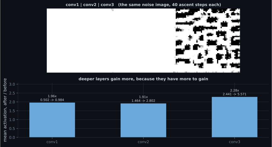
Layer	Activation before	After	Gain	Mean pixel change
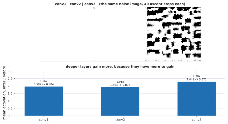
`conv1`	0.5019	0.9840	1.96×	0.5015
`conv2`	1.4643	2.8025	1.91×	0.5008
`conv3`	2.4411	5.5707	2.28×	0.4547

The receptive field is what changes across those rows. A conv1 unit sees a 3×3 pixel patch, so the only thing it can ask for is a favourable arrangement of nine pixels — repeated everywhere, which reads as texture. After two MaxPooling2D layers a conv3 unit sees a large region, so it can ask for a whole shape.

Note the last column: conv3 achieved the largest activation gain with the smallest pixel change (0.4547 against 0.5015). Deeper features are more specific, so satisfying them requires less indiscriminate rearranging.

Step size

figure conv3, 40 steps at each setting matplotlib

Gain improves steeply from 0.005 to 0.05 and then flattens, peaking at 2.41x at step 0.2 before falling back to 2.36x at 0.5. The dashed line explains it: mean pixel change is already 0.4800 at step 0.2 and only reaches 0.4887 at 0.5, because the clip absorbs everything extra. Past that point a larger step does not move the image further, it just moves it more coarsely.

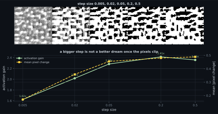
Step size	Activation after	Gain	Mean pixel change
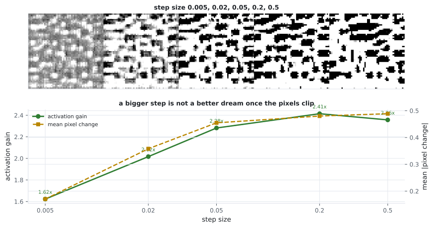
0.005	3.9614	1.62×	0.1705
0.020	4.9230	2.02×	0.3581
0.050	5.5707	2.28×	0.4547
0.200	5.8941	2.41×	0.4800
0.500	5.7537	2.36×	0.4887

This is a genuinely non-monotonic result and it is worth being precise about the cause. The gradient is recomputed at every step from the current image, so it is only valid locally. A step of 0.5 moves half the dynamic range on the strength of that local estimate, overshoots, and then spends the next step correcting — while the clip discards whatever went out of range. The measured gain at 0.5 is lower than at 0.2 despite moving the pixels further.

Practically: pick the step size by measuring the gain, not by eye. The visually “strongest” image here is not the one with the highest activation.

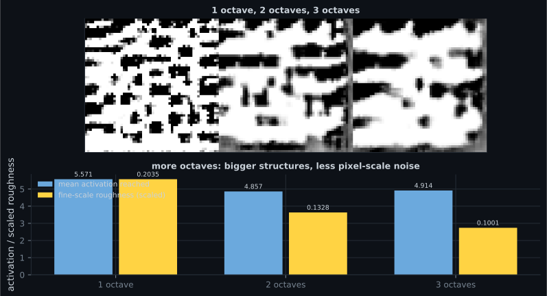
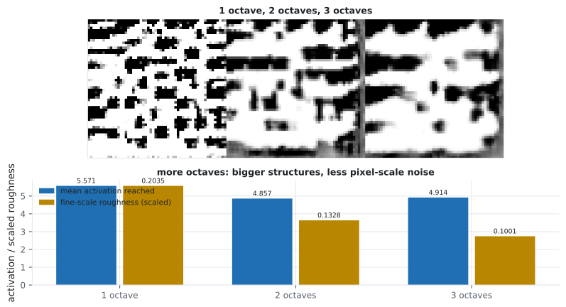
Octaves

The original DeepDream dreams at several resolutions, starting small and scaling up. The stated reason is that small images produce large features: at low resolution a fixed receptive field covers proportionally more of the picture.

Octaves	Activation reached	Fine-scale roughness
1	5.5707	0.2035
2	4.8568	0.1328
3	4.9144	0.1001

Be careful about what this does and does not show. Roughness halving is measured, and it means the multi-scale images contain less pixel-to-pixel noise. The usual claim that octaves produce larger structures is consistent with that but is not established by these two numbers — a smoother image is not automatically an image with bigger shapes, and measuring structure size properly needs something like a spatial autocorrelation length, which this module does not compute.

What is established: octaves cost activation and buy smoothness.

Dreaming across octaves

size = int(SIZE / OCTAVE_SCALE ** (octaves - 1))
current = tf.image.resize(base, (size, size)).numpy()
 
for octave in range(octaves):
    current = dream(layer, current, steps=STEPS // octaves)["image"]
    if octave + 1 < octaves:
        size = int(size * OCTAVE_SCALE)
        current = tf.image.resize(current, (size, size)).numpy()

Each upscale blurs what the previous octave produced, and the next round of ascent sharpens it again at the new resolution. The structure that survives is the structure the layer wanted at the coarser scale.

sketch Gradient ascent against descent p5.js

The same landscape, two rules. Click to place the dot, then press any key to take a step. Ascent climbs to a peak; descent runs to a valley.

Ascent from the left-hand starting point climbs the smaller peak and stops there — a local maximum. DeepDream has exactly this property, which is why running it twice from different noise gives two different images, and why a single dream should not be read as a complete picture of what a layer detects.

sketch The measured table, ranked p5.js

Click a column to rank every row by it. The bars are that column's values and the highest and lowest are computed from the numbers, not written in.

Pitfalls

Not normalising the gradient. Raw magnitudes differ by orders of magnitude between layers, so one step size cannot serve all of them.
Assuming a bigger step is a stronger dream. The gain peaked at 2.41× at step 0.2 and fell to 2.36× at 0.5, while pixel change barely moved (0.4800 → 0.4887).
Starting from a flat image. A constant has almost no gradient to amplify; start from noise.
Forgetting to clip. Out-of-range pixels inflate the activation without producing anything displayable.
Reading a dream as “what the layer detects”. It shows one local maximum reachable from one starting image, not the layer’s full preference.
Claiming octaves make bigger structures because the image looks smoother. Roughness fell 0.2035 → 0.1001, which is smoothness; structure size was not measured here.
Expecting published DeepDream imagery from a locally trained network. These features come from a 0.7767-accuracy Fashion-MNIST convnet, not from ImageNet.

Recap

DeepDream is gradient ascent on a layer’s activation with respect to the input image; the weights never change.
Normalising the gradient by its own standard deviation is what makes one step size valid across layers.
Depth selects scale: conv1 gained 1.96× as fine texture, conv3 gained 2.28× as coarse structure, with a smaller pixel change (0.4547 against 0.5015).
Gain against step size is non-monotonic — 1.62×, 2.02×, 2.28×, 2.41×, 2.36× — because clipping absorbs oversized steps.
Octaves traded activation for smoothness: 5.5707 → 4.9144 while roughness fell 0.2035 → 0.1001.
The result is a local maximum, so the starting noise selects the dream.

The same machinery — a frozen network, an image as the variable, gradient steps on a differentiable objective — becomes a style transfer engine as soon as the objective compares two images instead of maximising one number: Neural Style Transfer.

pch.quizTag pch.quizDefaultTitle

What is being optimised during DeepDream?

pch.quizShowAnswer

B — The input image, with the weights frozen — gradient ascent on a layer's activation with respect to the pixels — Nothing is trained. The gradient is taken with respect to the image, and the sign is positive because the goal is more activation, not less.
Why divide the gradient by its own standard deviation before each step?

pch.quizShowAnswer

B — Because raw gradient magnitudes differ by orders of magnitude between layers, so without it a single step size would be a tiny nudge at one depth and a saturated image at another — Normalising turns the step size into a fraction of the image's dynamic range, which is what makes gains comparable across layers.
conv1 produced fine texture while conv3 produced coarse structure. Why?

pch.quizShowAnswer

B — Receptive field — a conv1 unit sees a 3x3 patch, while a conv3 unit sees a large region after two pooling layers, so it can ask for a whole shape — Depth selects the spatial scale of what can be requested, which is the mechanism behind the visual difference between early- and late-layer dreams.
Activation gain rose from 1.62x to 2.41x as the step size grew from 0.005 to 0.2, then fell to 2.36x at 0.5. What causes the fall?

pch.quizShowAnswer

B — The gradient is only valid locally, so a very large step overshoots — and the clip discards whatever leaves the valid range, so the image barely moves further (0.4800 to 0.4887) — The number of steps was identical at every setting, so the step size chosen by measuring gain is not the largest available one.
Octaves reduced roughness from 0.2035 to 0.1001 but also reduced the activation reached, from 5.5707 to 4.9144. What is the honest conclusion?

pch.quizShowAnswer

B — Octaves measurably buy smoothness at the cost of activation; whether they produce larger structures was not measured here — A smoother image is not automatically an image with bigger shapes — establishing that would need a measurement of structure size, such as a spatial autocorrelation length.

🧪 Try It Yourself

pch.coffeeTagline

pch.coffeeCta

pch.feedbackHeading

pch.feedbackSubheading