Time Series Forecasting with RNNs

Forecasting is the one deep-learning task where a two-line baseline routinely beats a tuned network, and where the standard evaluation habits — random splits, MAE quoted without context, single-horizon results — quietly produce nonsense.

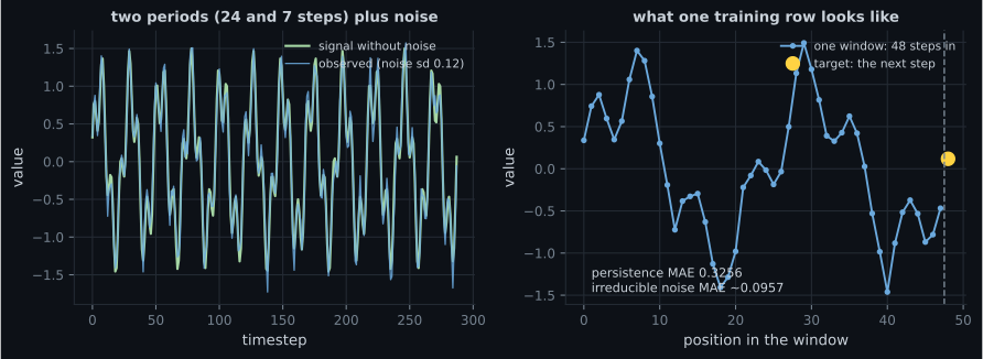
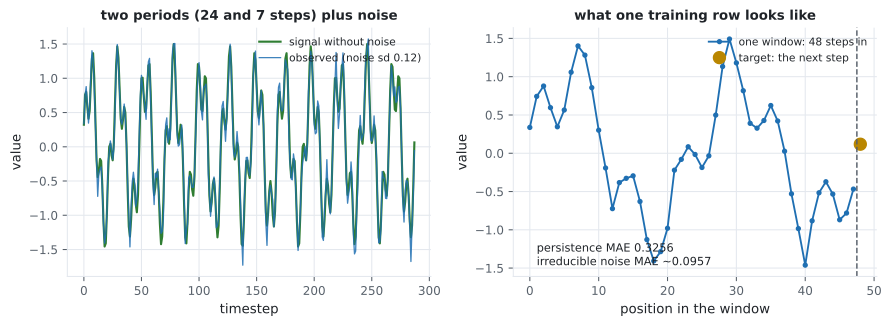
This page uses a generated series rather than a downloaded one, for a specific reason: the signal is known exactly, so the irreducible error is known too. Two periods (24 and 7 steps), Gaussian noise with $\sigma = 0.12$ . A perfect forecaster still scores MAE 0.0965 against the noisy target. Every number below is judged against that floor and against persistence.

What you’ll learn

How to turn one long series into supervised windows, and why the split must be chronological.
The two baselines that matter: persistence (MAE 0.3253) and predicting the training mean (0.6804).
The noise floor — $\sigma\sqrt{2/\pi} = 0.0965$ — and why a model near it is finished, not merely good.
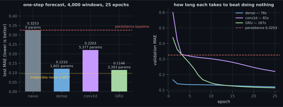
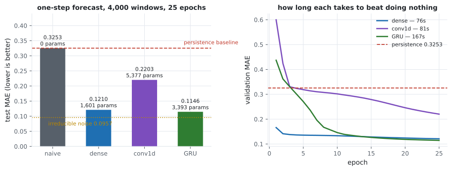
Four models measured: Dense 0.1210, Conv1D 0.2203, GRU 0.1146 at 1,601 / 5,377 / 3,393 parameters.
Why persistence gets better again at a 24-step horizon (1.3227 at 12, 0.6306 at 24).
Why a bidirectional layer is a bug in a forecaster, not an upgrade.

From one series to supervised rows

Windowing

def windows(series, timesteps=48, horizon=1):
    x = np.stack([series[i:i + timesteps] for i in range(len(series) - timesteps - horizon + 1)])
    y = series[timesteps + horizon - 1:]
    return x[..., None], y[:len(x)]          # (rows, timesteps, features), (rows,)

Each row is timesteps consecutive observations; the target is the value horizon steps after the window ends. The feature axis exists even for a univariate series — recurrent and convolutional layers both require (batch, time, features).

Two panels. Left: a noisy oscillating series in blue overlaid on the smooth noise-free signal in green, showing a repeating pattern with two interacting periods. Right: one 48-step window as a line of small markers with the target — the next step — highlighted as a large amber dot just beyond the window's edge, annotated with the persistence MAE of 0.3256 and the irreducible noise MAE of about 0.0958. — Generating the series is what makes the rest of the page honest: the green curve is the signal, the blue is what the model sees, and the gap between them is the error no model can remove. Target statistics: mean -0.0002, sd 0.7975, range [-1.728, 1.732].

The split has to respect time

python

cut = int(len(x) * 0.75)
x_train, y_train = x[:cut], y[:cut]      # everything before the cut
x_test, y_test = x[cut:], y[cut:]        # everything after

train_test_split(..., shuffle=True) on windowed data is leakage, and it is the single most common error in forecasting notebooks. Consecutive windows overlap by timesteps - 1 observations, so a shuffled split puts near-duplicates of test rows into training. The score that comes out is not wrong by a little.

Baselines first

Baseline	Test MAE
predict the training mean	0.6804
persistence — predict the last observed value	0.3253
the irreducible noise floor	0.0965

Persistence is one line — predicted = x_test[:, -1, 0] — and it is the number a model must beat to have justified its existence. The floor is the number that tells you when to stop tuning.

\text{MAE}_{\text{floor}} = \mathbb{E}\lvert \varepsilon \rvert = \sigma\sqrt{\tfrac{2}{\pi}} = 0.12 \times 0.7979 = 0.0958

(The measured 0.0965 is the sample estimate of that expectation.)

Four models, same windows

Model	Parameters	Test MAE	Beats persistence by	Seconds
persistence	0	0.3253	—	0.0
Dense(32)	1,601	0.1210	+0.2043	9.1
Conv1D ×2	5,377	0.2203	+0.1050	13.6
GRU(32)	3,393	0.1146	+0.2107	39.5

Two panels. Left: bars of test MAE for naive 0.3253, dense 0.1210, conv1d 0.2203 and GRU 0.1146, with a red dashed persistence line and an amber dotted irreducible-noise line near 0.096. Right: validation MAE per epoch, where dense drops below the persistence line within two epochs and flattens near 0.12, GRU crosses at epoch four and ends lowest, and conv1d is still descending at 0.22 after 25 epochs. — The GRU wins by 0.0064 over a flattened Dense layer while costing 4.3x the wall-clock and twice the parameters — and both sit close to the 0.0965 noise floor, so there was very little left to win. The Conv1D stack is the interesting failure: 5,377 parameters, still improving at epoch 25, and beaten by a single Dense layer. Its two pooling and convolution stages blur exactly the recent detail a one-step forecast depends on.

Three conclusions worth stating plainly:

A flattened Dense layer is a serious forecasting baseline. 1,601 parameters, nine seconds, and within 0.0064 of the GRU. On a 48-step window there is no long-range structure for recurrence to exploit.
The GRU wins, but the margin is tiny relative to its cost. +0.0064 MAE for 4.3× the training time. If a Dense model is within a hair of the noise floor, the architecture question is already answered.
Conv1D lost badly here. Convolution assumes the useful pattern is local and translation-invariant along time; a one-step forecast mostly depends on the last few observations, and pooling averages them away. Dilated causal convolutions (WaveNet-style) exist precisely to fix this — no pooling, exponentially growing receptive field, and the last timestep never blurred.

The horizon changes which baseline is hard

Horizon	Persistence MAE	GRU MAE	GRU advantage
1	0.3253	0.1146	+0.2107
6	0.9296	0.1161	+0.8135
12	1.3227	0.1134	+1.2094
24	0.6306	0.1078	+0.5228

A line chart of test MAE against forecast horizon. The red persistence line rises from 0.3253 at horizon 1 to a peak of 1.3227 at horizon 12 and falls to 0.6306 at horizon 24. The green GRU line is flat between 0.1078 and 0.1161 across all four horizons, just above a dotted irreducible-noise line at 0.0965. — Two things happen here and neither is the textbook story. Persistence peaks at horizon 12 — half of the 24-step period, where the series is maximally out of phase with itself — and recovers at 24, a full period later. The GRU is flat at ~0.11 at every horizon, because this signal is deterministic apart from noise: once the period is learned, 24 steps ahead is no harder than one. Real series lose predictability with distance; a generated one does not, and that difference is exactly what makes this figure worth reading carefully.

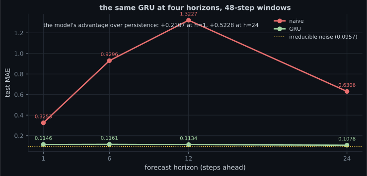
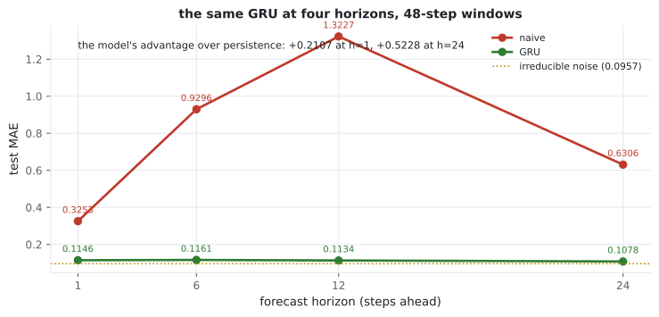
The generalisable lesson is about the baseline, not the model: persistence is a function of the series’ autocorrelation, so “we beat the naive baseline by 1.21 MAE” is a claim about the horizon you chose. Quote the baseline at every horizon you quote a model at.

diagram Diagram mermaid

  flowchart TB
  A["one long series"] --> B["window: 48 in, 1 target"]
  B --> C{"split"}
  C -->|"WRONG: shuffle"| D["overlapping windows leak
the test set into training"]
  C -->|"chronological"| E["train = past, test = future"]
  E --> F["baselines: mean 0.6804,
persistence 0.3253"]
  F --> G["model: Dense 0.1210,
GRU 0.1146"]
  G --> H{"near the noise
floor 0.0965?"}
  H -->|"yes"| I["stop — the rest is noise"]
  H -->|"no"| J["more capacity, longer window,
more features"]

Scaling, and the leak hiding inside it

Normalise with statistics from the training split only:

The only safe way to scale a series

mean = x_train.mean()                     # training rows only
std = x_train.std()
x_train = (x_train - mean) / std
x_test = (x_test - mean) / std            # the same numbers, not recomputed

Fitting the scaler on the whole series leaks the future’s mean and variance into training. It usually improves your reported score, which is what makes it dangerous.

For a series with a trend, differencing (np.diff) is often better than scaling: it removes the drift a fixed mean cannot follow, and it turns “predict the level” into “predict the change” — which also makes persistence the trivial prediction of zero.

What not to use

Idea	Why it fails on a forecaster
`Bidirectional(LSTM(...))`	the backward pass reads the future; at prediction time there is no future to read
Shuffled train/test split	overlapping windows leak; the score is meaningless
Scaler fitted on all data	the training rows learn the test period’s mean and variance
Accuracy as a metric	forecasting is regression — use MAE or RMSE and report the baseline
Reporting one horizon	persistence varies with the horizon; so does the apparent gain

sketch Windows, horizons and persistence p5.js

Drag along the series to move the window. The amber dot is the target and the grey dot is what persistence predicts; the gap between them is the error the baseline makes.

sketch The measured table, ranked p5.js

Click a column to rank every row by it. The bars are that column's values and the highest and lowest are computed from the numbers, not written in.

Pitfalls

A shuffled split. Consecutive windows overlap by 47 of 48 steps; shuffling puts near-copies of the test rows into training.
No baseline. Persistence scored 0.3253 here; a model reporting 0.30 would look fine and be worthless.
No noise floor. The best model reached 0.1146 against a floor of 0.0965 — 84% of the remaining error is irreducible, so further tuning buys almost nothing.
Scaling with statistics from the full series. It leaks the test period’s mean and variance and improves your reported score.
Bidirectional in a forecaster. It reads the future. It will validate beautifully and cannot be deployed.
Quoting one horizon. Persistence ranged from 0.3253 to 1.3227 across four horizons on the same data.
Assuming an RNN must beat a Dense layer. A flattened Dense(32) scored 0.1210 in 9 seconds against the GRU’s 0.1146 in 39.5.
Pooling in a Conv1D forecaster. It averages away the recent observations a short-horizon forecast leans on — measured 0.2203, worse than the Dense layer.

Recap

Windowing turns one series into (rows, timesteps, features); the split must be chronological because windows overlap.
Baselines on this series: training mean 0.6804, persistence 0.3253, irreducible noise 0.0965.
Measured at 25 epochs: Dense 0.1210 (1,601 params, 9.1s), Conv1D 0.2203 (5,377 params), GRU 0.1146 (3,393 params, 39.5s).
Persistence peaked at horizon 12 (1.3227 — half the 24-step period) and improved at 24 (0.6306); the GRU stayed flat near 0.11 because the generated signal never becomes unpredictable.
Scale with training-split statistics only; difference the series if it has a trend.
Never use a bidirectional layer, a shuffled split, or an accuracy metric in a forecaster.

Dropout, stacking and bidirectional layers — including which of them a forecaster may use — are next: Advanced Recurrent Layers.

pch.quizTag pch.quizDefaultTitle

Why is train_test_split(..., shuffle=True) wrong for windowed time series?

pch.quizShowAnswer

B — Because consecutive windows overlap by timesteps-1 observations, so shuffling puts near-duplicates of test rows into training — the score measures memorisation — The split must be chronological: train on the past, test on the future, exactly as deployment will work.
The best model scored MAE 0.1146 and the noise floor is 0.0965. What does that tell you?

pch.quizShowAnswer

B — Roughly 84% of the remaining error is irreducible noise, so further tuning has very little left to win — sigma*sqrt(2/pi) is the MAE a perfect forecaster still pays against a noisy target. Without it you cannot tell a finished model from a lazy one.
Persistence scored 0.3253 at horizon 1, 1.3227 at horizon 12 and 0.6306 at horizon 24. Why the non-monotonic shape?

pch.quizShowAnswer

B — Persistence tracks the series' autocorrelation: horizon 12 is half of the 24-step period, where the series is most out of phase with itself, and 24 is a full period later — Which is why 'we beat the naive baseline by 1.21' is a statement about the chosen horizon, not about the model.
A flattened Dense(32) scored 0.1210 against the GRU's 0.1146, in a quarter of the time. What follows?

pch.quizShowAnswer

B — On a 48-step window with no long-range structure, recurrence has little to add — the Dense model is a serious baseline and the GRU's +0.0064 has to justify 4.3x the cost — Recurrence pays off when the useful information is far back and order-dependent, which a 48-step periodic window barely provides.
Why must a forecasting model never use Bidirectional?

pch.quizShowAnswer

B — The backward pass reads later timesteps — at prediction time those are the future, so the model validates well and cannot be deployed — It is the same class of error as a shuffled split or a scaler fitted on all data: information that will not exist at inference time.

🧪 Try It Yourself

pch.coffeeTagline

pch.coffeeCta

pch.feedbackHeading

pch.feedbackSubheading