What you’ll learn

• the four cells — TP, FP, FN, TN — and how to stop confusing the middle two
• every common metric written as a ratio of those cells
• the ten-row example computed by hand, cell by cell
• scikit-learn’s row/column convention, and why people read the matrix backwards
• how to read a multiclass matrix, where the off-diagonal is the interesting part
• why the matrix is the only summary that loses nothing

Intuition

A single accuracy number compresses every prediction into one figure and throws away which kind of mistake was made. For most real problems the kinds are not interchangeable: telling a healthy patient they may be ill costs an anxious week, and telling an ill patient they are healthy can cost much more.

The confusion matrix keeps them separate. For a binary problem it is four numbers, and every metric in this phase is a ratio of some of them. It is the last point in the evaluation pipeline where no information has been discarded.

The math

Every metric, as a ratio of cells:

Note which cell each denominator uses:

• Precision divides by everything the model called positive — a column of the matrix.
• Recall divides by everything that actually is positive — a row.

That single distinction is the source of most confusion between them, and it is worth memorising as “precision is a column, recall is a row”.

Balanced accuracy

The average of per-class recall. On the 2%-positive problem from Introduction to Classification, a constant “always negative” model scores 0.98 accuracy and exactly 0.50 balanced accuracy — which is the number you actually wanted.

Worked example by hand

The ten-row example from the introduction, at threshold 0.5:

Step 1 — tally. TP = 4, FP = 2, FN = 1, TN = 3. They sum to 10, as they must.

Step 2 — assemble the matrix.

Step 3 — every metric, from those four numbers.

Six numbers describing one set of ten predictions, ranging from 0.60 to 0.80. Choosing which to report is a decision about what the model is for, not a technicality.

Step 4 — move the threshold to 0.65 and recount. Now rows 1–4 are predicted spam:

The model has not changed. One number in a comparison changed, and precision went up while recall went down. That trade-off is the subject of the next page.

See it move

Steps 1 to 4 by hand, for every threshold at once. Drag the threshold line through the ten scores and watch rows cross it: each crossing moves exactly one row from one cell of the matrix to another, and the six metrics recompute from the four counts.

Two things the static table cannot show. Only one row moves at a time. Sliding from 0.5 to 0.65 crosses row 6 alone, which is why exactly one cell pair changed in step 4 — the matrix moves in integer steps, and with ten rows every metric is quantised to tenths and sixths. Above 0.95 nothing is predicted spam, so precision is $0/0$: undefined, and scikit-learn will emit UndefinedMetricWarningUndefinedMetricWarning and substitute 0.0 unless you pass zero_divisionzero_division. A metric that can be undefined is a metric you should not average over folds without checking.

Reading a real matrix

figureBinary and ten-class matrices from real modelsmatplotlib

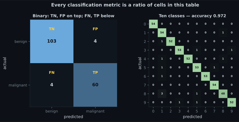
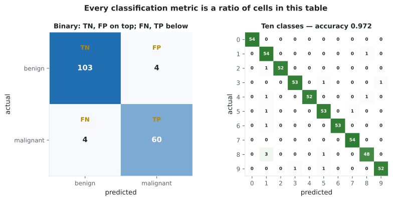
Reading the plot

The binary matrix (TN 103, FP 4, FN 4, TP 60):

• Accuracy is $(103+60)/171 = 0.953$.
• Precision is $60/64 = 0.938$ and recall is $60/64 = 0.938$ — equal only because FP happens to equal FN here. That is a coincidence, not a property.
• The four false negatives are the cells that matter clinically: four malignant tumours the model called benign.

The ten-class matrix:

• The diagonal is the correct predictions and dominates, as it should at 97% accuracy.
• The off-diagonal is the interesting part. Row 8 shows three eights predicted as ones — a specific, repeatable confusion, not random error.
• Reading a row tells you what a class gets mistaken for; reading a column tells you what gets mistaken for that class. Both are actionable in ways an accuracy score is not.

from sklearn.datasets import load_breast_cancer
from sklearn.linear_model import LogisticRegression
from sklearn.metrics import classification_report, confusion_matrix
from sklearn.model_selection import train_test_split
from sklearn.pipeline import make_pipeline
from sklearn.preprocessing import StandardScaler
 
X, y = load_breast_cancer(return_X_y=True)
y = 1 - y                       # 1 = malignant
X_tr, X_te, y_tr, y_te = train_test_split(
    X, y, test_size=0.3, random_state=0, stratify=y
)
 
model = make_pipeline(StandardScaler(), LogisticRegression(max_iter=5000))
model.fit(X_tr, y_tr)
pred = model.predict(X_te)
 
cm = confusion_matrix(y_te, pred)
print(cm)
# [[103   4]
#  [  4  60]]
 
tn, fp, fn, tp = cm.ravel()      # the standard unpacking idiom
print(f"TN={tn} FP={fp} FN={fn} TP={tp}")   # TN=103 FP=4 FN=4 TP=60
 
print(classification_report(y_te, pred, target_names=["benign", "malignant"]))

from sklearn.datasets import load_breast_cancer
from sklearn.linear_model import LogisticRegression
from sklearn.metrics import classification_report, confusion_matrix
from sklearn.model_selection import train_test_split
from sklearn.pipeline import make_pipeline
from sklearn.preprocessing import StandardScaler
 
X, y = load_breast_cancer(return_X_y=True)
y = 1 - y                       # 1 = malignant
X_tr, X_te, y_tr, y_te = train_test_split(
    X, y, test_size=0.3, random_state=0, stratify=y
)
 
model = make_pipeline(StandardScaler(), LogisticRegression(max_iter=5000))
model.fit(X_tr, y_tr)
pred = model.predict(X_te)
 
cm = confusion_matrix(y_te, pred)
print(cm)
# [[103   4]
#  [  4  60]]
 
tn, fp, fn, tp = cm.ravel()      # the standard unpacking idiom
print(f"TN={tn} FP={fp} FN={fn} TP={tp}")   # TN=103 FP=4 FN=4 TP=60
 
print(classification_report(y_te, pred, target_names=["benign", "malignant"]))

Multiclass

For $K$ classes the matrix is $K \times K$: entry $(i, j)$ counts samples of true class $i$ predicted as class $j$. There is no single TP or FP any more — each class gets its own, computed one-versus-rest:

• $TP_c$ is the diagonal entry for class $c$
• $FN_c$ is the rest of row $c$ (true $c$, predicted something else)
• $FP_c$ is the rest of column $c$ (predicted $c$, actually something else)
• $TN_c$ is everything else

Per-class metrics are then averaged, and the averaging choice matters:

On an imbalanced problem macromacro and weightedweighted can differ enormously. A model that is excellent on the common classes and useless on the rare ones scores well on weightedweighted and badly on macromacro — and macromacro is usually the honest one.

import numpy as np
from sklearn.datasets import load_digits
from sklearn.linear_model import LogisticRegression
from sklearn.metrics import confusion_matrix, f1_score
from sklearn.model_selection import train_test_split
from sklearn.pipeline import make_pipeline
from sklearn.preprocessing import StandardScaler
 
digits = load_digits()
X_tr, X_te, y_tr, y_te = train_test_split(
    digits.data, digits.target, test_size=0.3, random_state=0, stratify=digits.target
)
 
model = make_pipeline(StandardScaler(), LogisticRegression(max_iter=5000))
model.fit(X_tr, y_tr)
pred = model.predict(X_te)
 
cm = confusion_matrix(y_te, pred)
print(f"accuracy      {model.score(X_te, y_te):.4f}")        # 0.9722
print(f"macro F1      {f1_score(y_te, pred, average='macro'):.4f}")
print(f"weighted F1   {f1_score(y_te, pred, average='weighted'):.4f}")
 
# Where does the model actually go wrong?
errors = cm.copy()
np.fill_diagonal(errors, 0)
for true_c, pred_c in zip(*np.where(errors >= 2)):
    print(f"{errors[true_c, pred_c]} samples: true {true_c} -> predicted {pred_c}")
 
# 3 samples: true 8 -> predicted 1

import numpy as np
from sklearn.datasets import load_digits
from sklearn.linear_model import LogisticRegression
from sklearn.metrics import confusion_matrix, f1_score
from sklearn.model_selection import train_test_split
from sklearn.pipeline import make_pipeline
from sklearn.preprocessing import StandardScaler
 
digits = load_digits()
X_tr, X_te, y_tr, y_te = train_test_split(
    digits.data, digits.target, test_size=0.3, random_state=0, stratify=digits.target
)
 
model = make_pipeline(StandardScaler(), LogisticRegression(max_iter=5000))
model.fit(X_tr, y_tr)
pred = model.predict(X_te)
 
cm = confusion_matrix(y_te, pred)
print(f"accuracy      {model.score(X_te, y_te):.4f}")        # 0.9722
print(f"macro F1      {f1_score(y_te, pred, average='macro'):.4f}")
print(f"weighted F1   {f1_score(y_te, pred, average='weighted'):.4f}")
 
# Where does the model actually go wrong?
errors = cm.copy()
np.fill_diagonal(errors, 0)
for true_c, pred_c in zip(*np.where(errors >= 2)):
    print(f"{errors[true_c, pred_c]} samples: true {true_c} -> predicted {pred_c}")
 
# 3 samples: true 8 -> predicted 1

Two lines of NumPy turn a wall of numbers into one actionable sentence: this model confuses eights with ones, and nothing else systematically.

Which cell should you be optimising?

No metric knows your costs, so this is a routing question you answer before choosing one:

  flowchart TD
  A["Which mistake hurts more?"] --> B{"A missed positive
-- FN"}
  A --> C{"A false alarm
-- FP"}
  A --> H{"Both, and you can
price them"}
  A --> J{"Genuinely unsure,
classes balanced"}
  B -->|"cancer screening,
fraud, safety"| D["Maximise recall.
Accept low precision."]
  D --> E["Lower the threshold.
Report recall at a
fixed false-positive budget."]
  C -->|"spam, auto-blocking,
customer contact"| F["Maximise precision.
Accept low recall."]
  F --> G["Raise the threshold.
Report precision at a
fixed recall floor."]
  H -->|"each error has
a price in currency"| I["Skip ratio metrics.
Minimise expected cost --
it names the threshold directly."]
  J --> K["F1 or balanced accuracy
as a placeholder,
declared as a placeholder."]

The branch most teams skip is the third. If a false positive costs €4 of wasted review and a false negative costs €300 of loss, no ratio of counts is the right objective — expected cost is, and it implies a threshold of $t^* = C_{FP} / (C_{FP} + C_{FN})$ without any tuning. That derivation is on Cost-Sensitive Learning and Decision Thresholds.

Fill this row in for your own problem before you choose a metric. If you cannot say which error is worse, you do not yet know what the model is for.

Pitfalls

🧪 Try It Yourself

Exercise 1 – Count the four cells

Exercise 2 – Derive six metrics from four numbers

Exercise 3 – Unpack a scikit-learn matrix

Exercise 4 – Watch the cells move with the threshold

Exercise 5 – Find the systematic multiclass confusion

Recap

• Four cells: TP, FP, FN, TN. Read the second word first — a false positive is a false alarm, a false negative is a miss.
• Precision divides by a column (everything predicted positive); recall divides by a row (everything actually positive).
• The ten-row example: TN 3, FP 2, FN 1, TP 4 → accuracy 0.700, precision 0.667, recall 0.800, specificity 0.600, $F_1$ 0.727.
• Moving the threshold to 0.65 gives precision 0.750 and recall 0.600, with no retraining.
• scikit-learn puts actual on rows and predicted on columns; cm.ravel()cm.ravel() is TN, FP, FN, TP.
• In multiclass the off-diagonal is the diagnosis, and the averaging mode is part of the claim.

Exercise 6 – Tabulate every threshold at once

Next

Continue to Precision, Recall, and F1-Score — which of these four cells you are willing to trade, and how to pick a threshold that reflects the answer.