
Capstone 3 - Demand Forecasting for Ordering
The decision
Section titled “The decision”A warehouse orders tomorrow’s stock tonight. Two things can go wrong:
- Understock. A unit of unmet demand costs 9 — a lost sale plus the expedited replacement.
- Overstock. A unit held overnight costs 1 — space, capital and spoilage risk.
Nobody in this problem wants a forecast. They want a quantity, and the forecast is an intermediate value on the way to it. That distinction is the whole capstone, and it changes both the model and the metric.
This project composes:
- the series and lag features from Time Series Forecasting Fundamentals
- the cost-derived operating point from Cost-Sensitive Learning
- the honest-baseline discipline from Experiment Tracking
The data and the baseline
Section titled “The data and the baseline”The same 1,096-day series: trend, weekly and yearly seasonality, and AR(1) noise with sd 8.43 against the series’ 30.91. A chronological 80/20 split gives 854 training days and 214 test days.
The features are lags 1, 2, 3, 7 and 14, rolling means of the past 7 and 28 days, day of week, and a time index — every one shifted so that no row sees its own target. Ridge on those features had MASE 0.561 on that page, which is where this capstone starts.
Ordering the forecast is the expensive option
Section titled “Ordering the forecast is the expensive option”The obvious policy is order what you expect to sell:
order = ridge.predict(X_test)                     # order the point forecast

short = np.maximum(actual - order, 0)
over = np.maximum(order - actual, 0)
cost = 9 * short.sum() + 1 * over.sum()
print(f"{cost:,.0f}") # 6,382| Policy | Units short | Units over | Total cost |
|---|---|---|---|
| order = point forecast | 615 | 845 | 6,382 |
A point forecast is (approximately) the conditional mean, so it is above demand about half the time and below it about half the time. When the two errors cost 9 and 1, being below half the time is a catastrophe: those 615 short units cost 5,537 of the 6,382 total.
The newsvendor result
Section titled “The newsvendor result”The fix is the same derivation as the classification threshold, one page over. Order ; the marginal unit is worth ordering while the expected cost of not having it exceeds the expected cost of holding it:
so the optimal order is the quantile of the demand distribution at
This is the classical newsvendor solution, and it says something useful about modelling: you do not need a distribution, you need one quantile of it, and quantile regression estimates exactly that by minimising the pinball loss
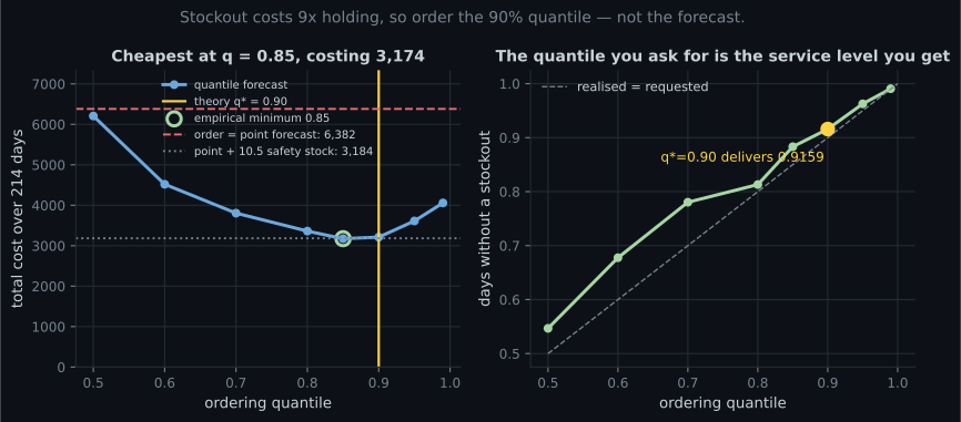
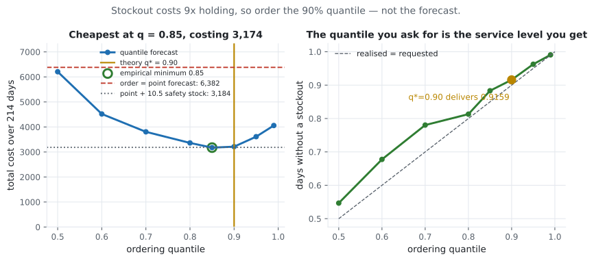
| Policy | Units short | Units over | Total cost |
|---|---|---|---|
| order = point forecast | 615 | 845 | 6,382 |
| point forecast + safety stock of 10.5 | 71 | 2,548 | 3,184 |
| linear quantile regression at | 75 | 2,538 | 3,212 |
| quantile gradient boosting at | 153 | 2,889 | 4,267 |
| oracle: order exactly the demand | 0 | 0 | 0 |
Four readings.
Asking the right question halved the cost. 6,382 → 3,212 with no change to the features, the model family or the amount of data. The improvement came from replacing “predict demand” with “predict the 0.90 quantile of demand”.
A tuned safety stock is just as good here — and needs data to tune. The buffer of 10.5 units was
chosen by minimising cost on the last 20% of the training window, and it landed at 3,184, within 1% of
the quantile model. That is an honest result and a useful one: on a series with roughly constant
forecast error, forecast + constant is a fine policy. The quantile model earns its keep when the error
is heteroscedastic — busier days are less predictable — because it can widen the buffer where the
uncertainty is, and it needs no separate tuning step.
Trees lose again, for the same reason as before. Quantile gradient boosting reached only 4,267, because a tree’s prediction is bounded by the training targets and this series trends upward at 0.06 per day. The same finding appeared in Phase 10: extrapolation is a model-class property, and no loss function fixes it.
The service level is the deliverable. Requesting the 0.90 quantile produced stockout-free days on 0.9159 of the test window. That number — not MAE, not MASE — is what an operations team will hold you to, and it comes out of the model calibrated because the pinball loss is what was minimised.
See it move
Section titled “See it move”Two things move together here and it is worth watching them do it: the cost ratio you assume, and the quantile it implies. Drag the stockout cost and the sketch recomputes , snaps to the nearest measured quantile model, and shows the realised cost, the units short and over, and the service level you would have received across the 214 test days.
Set the ratio to 4:1 and becomes 0.80, costing 3,361; set it to 19:1 and is 0.95, costing 3,612. Both are worse than the 0.85–0.90 region, and both are still roughly half the 6,382 you pay for ordering the point forecast. That is the practical shape of this result: getting the cost ratio approximately right is worth far more than getting it exactly right, and getting the question right — a quantile rather than a mean — is worth more than either.
The engineering around it
Section titled “The engineering around it”Three things this project needs before it can run every night, all from Phase 11:
A point-in-time feature function. lag_frame shifts every column before use, so a row cannot see
its own target. Tonight’s order uses features as of tonight, which means the serving path must call the
same function with asof = today — and a parity test must prove it does.
A schema contract on the incoming series. The features are lags of one column, so the corruption that matters is a missing or late day. Assert: no gaps in the date index, no nulls in the last 28 days, and the latest value inside the fitted range. A missing day silently shifts every lag by one, which is the time-series version of a column reorder.
A cost-parameterised config, not a hard-coded quantile. q = c_under / (c_under + c_over) belongs in
the config next to the two costs, so that when finance revises the stockout cost the change is one
number and no retraining.
CONFIG = {"c_under": 9.0, "c_over": 1.0, "window": 28, "model": "quantile_linear"}


def nightly_order(series, model, config, asof):
    """Tonight's order quantity, plus everything an audit would ask for."""
    q = config["c_under"] / (config["c_under"] + config["c_over"])
    features = lag_frame(series).loc[[asof]]          # same function as training
    order = float(model.predict(features)[0])
    return {
        "asof": str(asof.date()),
        "order": round(order, 1),
        "quantile": q,
        "point_forecast": round(float(point_model.predict(features)[0]), 1),
        "implied_buffer": round(order - float(point_model.predict(features)[0]), 1),
        "config": config,
    }
Logging implied_buffer is the operational tell: if it drifts from its usual size, either the model’s
uncertainty estimate has changed or the input series has.
The nightly job, with the two guards that stop it ordering nonsense:
  flowchart TD
  CRON["nightly job, asof = today"] --> S[("daily sales series")]
  S --> V{{"schema contract:
no gaps in the date index,
no nulls in the last 28 days,
latest value in range"}}
  V -->|"a day is missing"| HALT["halt. a gap shifts every lag
by one -- the time-series
version of a column reorder"]
  V -->|"clean"| F["lag_frame(series).loc[[asof]]
the same function used in training"]
  CFG[("config:
c_under = 9, c_over = 1")] -->|"q = c_under / (c_under + c_over)"| Q{{"q = 0.90"}}
  F --> QM["quantile model at q"]
  Q --> QM
  F --> PM["point forecast model
-- for the diagnostic only"]
  QM --> ORD["order quantity"]
  PM --> IB["implied_buffer =
order minus point forecast"]
  ORD --> LOG["log order, quantile,
point forecast, implied_buffer,
and the config that produced them"]
  IB --> LOG
  LOG --> WATCH{{"is implied_buffer near
its usual size?"}}
  WATCH -->|"drifted"| INV["either the model's uncertainty
changed or the series did.
Investigate before trusting
tonight's number."]
  WATCH -->|"normal"| SEND["send the order"]
  SEND --> OUT["next day: realised demand"]
  OUT --> SVC["track service level and
cost against the requested q"]
  SVC -.->|"if realised service level
drifts from q"| RETRAIN["refit. the quantile model
is only calibrated while
the error distribution holds"]
  RETRAIN -.-> QM
  FIN["finance revises the
stockout cost"] -.->|"one number, no retraining"| CFG
The dotted edge on the right is the one that distinguishes this from a forecasting project. The deliverable is not the forecast, it is the order, and the feedback loop that keeps it honest compares the realised service level with the quantile that was requested — a check available every single day, with no model metric involved.
What this project does not solve
Section titled “What this project does not solve”- Lead time. The problem as posed is one day ahead. A three-day lead time needs the quantile of cumulative demand over three days, which is not three times the daily quantile.
- Perishability and multi-period effects. Overstock here is charged once. Real overstock either carries forward (reducing tomorrow’s order) or expires.
- Censored demand. The series records demand. Real data records sales, which are demand truncated by whatever was on the shelf, so training on sales after a stockout teaches the model that demand was lower than it was.
- Heteroscedastic gains, unmeasured. The argument that quantile regression beats a constant buffer when variance varies is a claim this dataset cannot support: its noise is homoscedastic by construction, and here the two policies tie at 3,212 against 3,184.
The last one is the honest headline for this capstone: on this series, a tuned constant buffer is as good as the quantile model. What the quantile model gives you is one fewer tuning step, a directly interpretable service level, and a policy that will still be right when the variance stops being constant.
- Ordering the point forecast cost 6,382 over 214 days: 615 units short, 845 over.
- The newsvendor quantile is .
- Ordering that quantile cost 3,212 — 75 short, 2,538 over — a 1.99× improvement from asking a different question of the same features.
- A tuned safety stock of 10.5 units cost 3,184: statistically the same, with an extra tuning step.
- Quantile gradient boosting reached only 4,267, because trees cannot extrapolate a trend.
- The realised service level was 0.9159 against the 0.9000 requested.
- The cost curve is flat between 0.85 and 0.90, so the cost ratio only needs to be roughly right.
-
A stockout costs 9 and a day of holding costs 1. What should tonight's order be?
The newsvendor solution. Measured here: 6,382 for the point forecast against 3,212 for the 0.90 quantile. Going further to 0.99 costs 4,058 — over-ordering has a price too.
pch.quizShowAnswer
B — The 0.90 quantile of the demand distribution — c_under / (c_under + c_over) — The newsvendor solution. Measured here: 6,382 for the point forecast against 3,212 for the 0.90 quantile. Going further to 0.99 costs 4,058 — over-ordering has a price too.
-
Why is ordering the point forecast so expensive when the two errors cost 9 and 1?
Nothing is wrong with the forecast; it answers a question nobody asked. Under asymmetric costs the useful output is a quantile, and quantile regression estimates it directly by minimising the pinball loss.
pch.quizShowAnswer
B — A point forecast is roughly the conditional mean, so it is below demand about half the time — and those 615 short units account for 5,535 of the 6,382 total cost — Nothing is wrong with the forecast; it answers a question nobody asked. Under asymmetric costs the useful output is a quantile, and quantile regression estimates it directly by minimising the pinball loss.
-
Your quantile model at q = 0.90 and a tuned constant safety stock cost 3,212 and 3,184. What do you conclude?
A 1% difference over 214 days is noise. Reporting the tie honestly is the right move; the quantile approach earns its keep when forecast error varies with the level, which this series does not test.
pch.quizShowAnswer
B — They are statistically indistinguishable on this series, whose noise is homoscedastic — the quantile model's advantages are one fewer tuning step and a directly interpretable service level — A 1% difference over 214 days is noise. Reporting the tie honestly is the right move; the quantile approach earns its keep when forecast error varies with the level, which this series does not test.
-
You requested the 0.90 quantile and 91.59% of test days had no stockout. What does that tell you?
That agreement is what makes a quantile forecast operationally useful. MAE and MASE describe the middle of the distribution; the service level describes the promise you are making.
pch.quizShowAnswer
B — The quantile estimate is calibrated: the service level you request is the one you receive, which is the number operations actually cares about — That agreement is what makes a quantile forecast operationally useful. MAE and MASE describe the middle of the distribution; the service level describes the promise you are making.
-
Quantile gradient boosting cost 4,267 against linear quantile regression's 3,212. Why?
It is the same finding as in Phase 10, where boosting reached MASE 0.670 against ridge's 0.561. Changing the loss function does not give a tree the ability to predict outside the range it has seen; differencing the series or adding a linear component does.
pch.quizShowAnswer
B — Trees cannot extrapolate: their predictions are bounded by the training targets, and this series' level rises 0.06 per day — It is the same finding as in Phase 10, where boosting reached MASE 0.670 against ridge's 0.561. Changing the loss function does not give a tree the ability to predict outside the range it has seen; differencing the series or adding a linear component does.
🧪 Try It Yourself
Section titled “🧪 Try It Yourself”Exercise 1 – Price the naive policy
Section titled “Exercise 1 – Price the naive policy”Exercise 2 – Order the newsvendor quantile
Section titled “Exercise 2 – Order the newsvendor quantile”Exercise 3 – Sweep the quantile
Section titled “Exercise 3 – Sweep the quantile”Exercise 4 – Compare against a tuned safety stock
Section titled “Exercise 4 – Compare against a tuned safety stock”Exercise 5 – Try the tree, and see it lose
Section titled “Exercise 5 – Try the tree, and see it lose”Capstone 4 - Ticket Triage with Text — from a quantity to a routing decision, where the model is allowed to abstain and the interesting metric is how much work it can take on at a given accuracy.
pch.coffeeTagline
pch.coffeeCtapch.feedbackHeading
pch.feedbackSubheading