Chapter 11 Worked Problems

#	problem	sections	the answer in one line
1	How do you choose $K$ ?	§11.5	held-out likelihood picks $3$ ; BIC $3$ ; AIC $4$ ; training $L$ picks $6$
2	What does a variance floor buy?	§11.2, §11.5	it does not remove the singularity; it prices it
3	How many optima does a fit have?	§11.3, §11.5	$K!$ copies of each, identical to $0.000\times10^{0}$
4	Can a density model classify?	§11.1, §11.4	$0.9650$ held out, the same as the fit that saw the labels
5	What does tying the variances cost?	§11.1, §11.5	$1.9542$ nats of fit; BIC and held-out $L$ then disagree
6	GMM against kernel density estimation	§11.5	$8$ stored numbers beat $600$ stored points by $13.7$ nats
7	Does held-out $L$ find the true $K$ as $N$ grows?	§11.5	BIC does; held-out $L$ starts over-selecting
8	What is $K$ when the data is not Gaussian?	§11.5	not a count — a budget

All eight share one setup. The data is drawn from a mixture whose parameters we know, so that “the right answer” exists and can be checked — the move page 1108 introduced.

setup.py

import numpy as np
 
TRUE_PI = np.array([0.45, 0.30, 0.25])
TRUE_MU = np.array([-3.0, 0.5, 4.0])
TRUE_VAR = np.array([0.8, 0.5, 1.2])
 
rng = np.random.default_rng(42)
ztr = rng.choice(3, 600, p=TRUE_PI)
DATA = rng.normal(TRUE_MU[ztr], np.sqrt(TRUE_VAR[ztr]))    # training
zte = rng.choice(3, 600, p=TRUE_PI)
TEST = rng.normal(TRUE_MU[zte], np.sqrt(TRUE_VAR[zte]))    # held out
 
def gauss(x, mu, var):
    return np.exp(-0.5 * (x - mu) ** 2 / var) / np.sqrt(2 * np.pi * var)
 
def resp(x, pi, mu, var):                   # Equation 11.17
    W = pi[None, :] * gauss(x[:, None], mu[None, :], var[None, :])
    return W / W.sum(1, keepdims=True)
 
def loglik(x, pi, mu, var):                 # Equation 11.10
    W = pi[None, :] * gauss(x[:, None], mu[None, :], var[None, :])
    return float(np.log(W.sum(1)).sum())
 
def em(x, K, seed, floor=1e-6, iters=500):  # Algorithm on page 1107
    r = np.random.default_rng(seed)
    pi = r.dirichlet(np.ones(K))
    mu = r.choice(x, K, replace=False)
    var = np.full(K, float(x.var()))
    prev = loglik(x, pi, mu, var)
    for _ in range(iters):
        R = resp(x, pi, mu, var)
        Nk = R.sum(0)
        if Nk.min() < 1e-12:                # page 1104's component death
            break
        mu = (R * x[:, None]).sum(0) / Nk               # Equation 11.54
        v = (R * (x[:, None] - mu[None, :]) ** 2).sum(0) / Nk
        var = np.maximum(v, floor)                      # Equation 11.55
        pi = Nk / len(x)                                # Equation 11.56
        cur = loglik(x, pi, mu, var)
        if abs(cur - prev) < 1e-10 * max(1.0, abs(cur)):
            break
        prev = cur
    return pi, mu, var, loglik(x, pi, mu, var)
 
def best_em(x, K, tries=12, seed0=0):
    """Page 1102 measured 17 distinct optima on 7 points. Restart."""
    best = None
    for t in range(tries):
        c = em(x, K, seed0 + t)
        if best is None or c[3] > best[3]:
            best = c
    return best

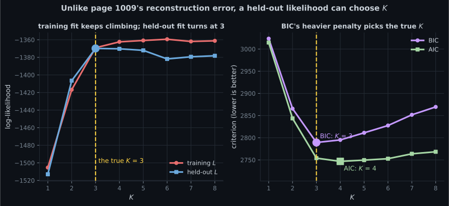
Problem 1 — How do you choose K?

Statement. §11.5 opens with “throughout this chapter, we assumed that the number of components $K$ is known. In practice, this is often not the case”, points at nested cross-validation in one sentence, and stops. Run it. Page 1009 found that Chapter 10’s analogue — held-out reconstruction error — cannot choose $M$ , because it falls monotonically to zero on any data at all. Does the same failure hit Chapter 11?

Method. Fit $K = 1 \dots 8$ on $600$ points, score each fit on a separate $600$ points, and alongside those compute BIC $= -2L + q\log N$ and AIC $= -2L + 2q$ , where $q = 3K - 1$ is the free parameter count ( $K$ means, $K$ variances, $K-1$ free weights).

problem_1.py

n = len(DATA)
print(f"{'K':>3} {'params':>7} {'train L':>12} {'held-out L':>12} "
      f"{'BIC':>12} {'AIC':>12}")
for K in range(1, 9):
    pi, mu, var, L = best_em(DATA, K)
    q = 3 * K - 1
    print(f"{K:>3} {q:>7} {L:>12.4f} {loglik(TEST, pi, mu, var):>12.4f} "
          f"{-2*L + q*np.log(n):>12.4f} {-2*L + 2*q:>12.4f}")

text

  K  params      train L   held-out L          BIC          AIC
  1       2   -1505.3457   -1512.9788    3023.4853    3014.6914
  2       5   -1416.8173   -1406.5088    2865.6192    2843.6346
  3       8   -1369.0609   -1369.8615    2789.2973    2754.1219
  4      11   -1362.3691   -1370.2832    2795.1044    2746.7381
  5      14   -1360.8031   -1372.0447    2811.1632    2749.6062
  6      17   -1359.4053   -1381.8189    2827.5583    2752.8105
  7      20   -1361.9098   -1379.3394    2851.7581    2763.8195
  8      23   -1361.1949   -1378.1859    2869.5192    2768.3898

Answer. Unlike Chapter 10’s reconstruction error, the held-out likelihood does turn around — and it turns around at the true $K = 3$ .

criterion	picks	why
training $L$	$6$	it can only rise; it stops at $6$ because EM stopped, not because $7$ is worse
held-out $L$	$\mathbf{3}$	a density too flexible assigns less probability to data it has not seen
BIC	$\mathbf{3}$	$\log N = 6.397$ per parameter, a heavy penalty
AIC	$4$	$2$ per parameter, a light one

The difference from page 1009 is structural, not a matter of luck. Reconstruction error asks how close does the model get to this point, and a bigger subspace can never project a point further away, so held-out error falls forever. A likelihood asks how much probability mass does the model put here, and mass is conserved — $\int p(x)\,dx = 1$ . Spending it on a bump the training set happened to show and the test set does not is a loss that shows up immediately. Normalisation is what makes held-out scoring work.

Note that the training column at $K=7$ is below $K=6$ ( $-1361.9098$ against $-1359.4053$ ). That is not a counterexample to monotonicity — a $7$ -component model contains every $6$ -component one, so its supremum is higher. It is EM failing to find it in $12$ restarts, which is page 1102’s multimodality showing up as a measurement artefact.

Left, two curves against K from one to eight: a red training curve rising and flattening, and a blue held-out curve that peaks at K equals three and then falls, with a dashed vertical line at three. Right, BIC and AIC curves, both dropping steeply then rising, with BIC's minimum on the dashed line at three and AIC's one step to its right at four. — The blue curve is the whole point: it comes back down. Page 1009's held-out reconstruction error never did, on any data. AIC's lighter penalty buys one component too many, which is the behaviour it is known for.

Problem 2 — What does a variance floor buy?

Statement. Page 1102 measured Equation 11.10 reaching $+16.377668$ at $\sigma^2 = 10^{-30}$ : the likelihood is unbounded above, and every practical implementation — including this page’s em — hides that behind np.maximum(v, floor). §11.5 names the problem exactly — “this happens when the mean of a mixture component is identical to a data point and the covariance tends to $0$ ” — and suggests a Bayesian prior on the parameters instead of a fix. What exactly does a floor do, and how should one be chosen?

Method. Fit $K = 6$ to only $60$ points, which is enough components and few enough points that collapse is common. Run $200$ random starts at each of eight floors, with $4000$ iterations so that a collapsing component has time to reach the floor. Record how often the floor is active (some component’s variance sits on it), the best log-likelihood found, and the best found among runs the floor never touched.

problem_2.py

SMALL = DATA[:60]
print(f"sample variance of the 60 points: {SMALL.var():.6f}")
print(f"{'floor':>10} {'floor active':>14} {'best L':>12} "
      f"{'best L, floor idle':>20} {'min var found':>15}")
floors = [1e-12, 1e-10, 1e-8, 1e-6, 1e-4, 1e-3, 1e-2, 1e-1]
bests = []
for fl in floors:
    Ls, mins = [], []
    for t in range(200):
        pi, mu, var, L = em(SMALL, 6, 3000 + t, floor=fl, iters=4000)
        Ls.append(L)
        mins.append(float(var.min()))
    Ls, mins = np.array(Ls), np.array(mins)
    active = mins <= fl * (1 + 1e-9)
    idle = Ls[~active]
    bests.append(Ls.max())
    print(f"{fl:>10.0e} {int(active.sum()):>11}/200 {Ls.max():>12.4f} "
          f"{(idle.max() if len(idle) else float('nan')):>20.4f} "
          f"{mins.min():>15.3e}")
 
print(f"slope of best L against log10(floor) : "
      f"{np.polyfit(np.log10(floors), bests, 1)[0]:.4f} nats per decade")
print(f"one decade of a collapsed component  : "
      f"{0.5*np.log(10):.4f} nats")

text

sample variance of the 60 points: 8.780058
     floor   floor active       best L   best L, floor idle   min var found
     1e-12           1/200    -120.9761            -124.6420       1.000e-12
     1e-10           1/200    -123.2786            -124.6420       1.000e-10
     1e-08           1/200    -124.6420            -124.6420       1.000e-08
     1e-06           1/200    -124.6420            -124.6420       1.000e-06
     1e-04          10/200    -125.3425            -128.9013       1.000e-04
     1e-03          15/200    -127.3459            -128.9013       1.000e-03
     1e-02          13/200    -128.9013            -128.9013       1.000e-02
     1e-01         200/200    -133.2236                  nan       1.000e-01
slope of best L against log10(floor) : -0.8594 nats per decade
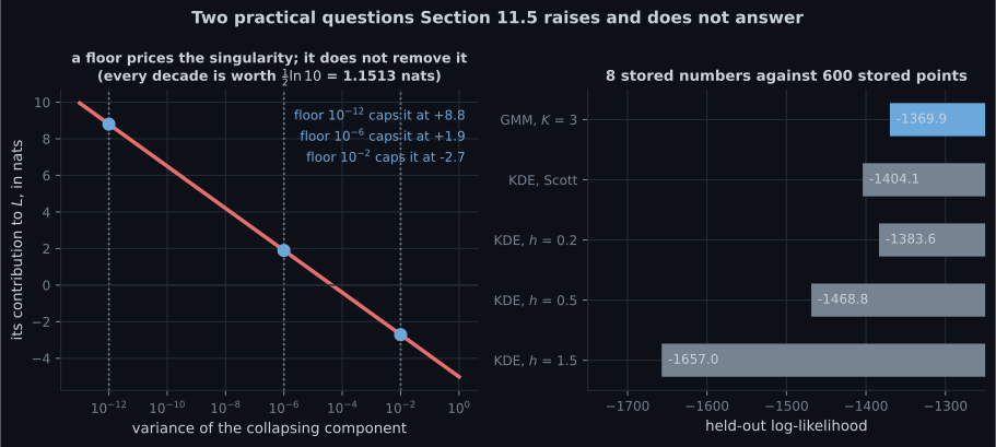
one decade of a collapsed component  : 1.1513 nats

Answer. The floor does not remove the singularity. It sets a price for it, and the price is exactly $\tfrac12\ln 10 = 1.1513$ nats per decade.

Read the top two rows: $-120.9761$ at $10^{-12}$ and $-123.2786$ at $10^{-10}$ . The difference is $2.3025$ over two decades, or $1.15125$ per decade — $\ln 10 / 2$ to five significant figures. That is not a coincidence; it is arithmetic. A component that has collapsed onto a single point $x_j$ with weight $\pi_k$ contributes

\log \pi_k \mathcal{N}(x_j \mid x_j, \sigma_k^2) = \log \pi_k - \tfrac12\log(2\pi\sigma_k^2),

so lowering $\sigma_k^2$ by a factor of ten always adds the same $\tfrac12\ln 10$ . The floor is the only thing standing between Equation 11.10 and $+\infty$ , and every decade you give it is worth the same fixed amount.

Left, a straight red line on a logarithmic horizontal axis rising steadily as the variance falls from one to ten to the minus thirteen, with three dotted vertical lines marking floors at ten to the minus twelve, minus six and minus two, each carrying a blue dot and its capped value. Right, five horizontal bars of held-out log-likelihood, the shortest and best a blue bar labelled GMM with eight stored numbers, the other four grey KDE bars each storing six hundred points. — The left line is straight because the divergence is logarithmic: each decade of variance is worth exactly half the natural log of ten. The right panel's best KDE stores six hundred points to finish 13.7 nats behind eight numbers, and its bandwidth moves the score by 273 nats — more than the entire K sweep of problem 1.

The rest of the table says something less obvious and more useful. The floor that produces the best honest fit is a large one.

floor	what the winner looks like
$10^{-12}$ to $10^{-6}$	the top score belongs to a run with a component of essentially zero width — a spike on one point, $-124.6420$ or better
$10^{-4}$ to $10^{-2}$	the spikes are capped low enough to stop winning; the genuine six-component fit, $-128.9013$ , takes the top spot
$10^{-1}$	the constraint binds in all $200$ runs and the best score falls to $-133.2236$ — the floor is now above real component widths

The best L, floor idle column is the one to watch. At floors of $10^{-6}$ and below it reads $-124.6420$ , which looks like a clean non-degenerate fit but is not: those runs simply have a component narrow enough to escape the floor’s notice while still being a spike. Once the floor rises to $10^{-4}$ that column drops to $-128.9013$ , and that is what a real six-component fit of these sixty points scores. The floor was not just capping the singularity — it was concealing how many runs had fallen into it.

The overall regression slope, $-0.8594$ nats per decade, is shallower than the $-1.1513$ the collapsed branch predicts, which is the same fact from the other side: over most of the range the best run is not a collapsed one, so the trend is a blend of the singular branch and a flat honest one.

A floor is a hard constraint with no principle behind it, and the table shows both failure modes: too small and it lets spikes win, too large and it distorts real components. A rule of thumb that works here is $10^{-2}$ to $10^{-3}$ times the sample variance — with $\mathrm{Var} = 8.780058$ that gives $10^{-2}$ to $10^{-1}$ , and $10^{-2}$ is indeed the largest floor in the table that has not started costing anything.

§11.5’s Bayesian suggestion is better because it is continuous. An inverse-gamma prior on $\sigma_k^2$ — the conjugate choice, though §11.5 correctly notes the joint model has no conjugate prior — adds $-(\alpha+1)\log\sigma_k^2 - \beta/\sigma_k^2$ to the objective, and the $-\beta/\sigma_k^2$ term goes to $-\infty$ faster than the $-\tfrac12\log\sigma_k^2$ gain goes to $+\infty$ . The singularity is removed rather than capped, and the M-step stays closed-form.

Problem 3 — How many optima does a fit have?

Statement. Page 1102 found $17$ distinct optima on $7$ points and called them distinct. Some of them are not. §11.3 writes the update equations in terms of an index $k$ that has no meaning of its own. What follows from that?

Method. Fit $K = 3$ , then evaluate Equation 11.10 at all $3! = 6$ relabellings of the fitted parameters.

problem_3.py

import itertools
 
pi, mu, var, L = best_em(DATA, 3)
vals = []
for perm in itertools.permutations(range(3)):
    p = list(perm)
    vals.append(loglik(DATA, pi[p], mu[p], var[p]))
vals = np.array(vals)
 
print(f"fitted means, sorted : {np.round(np.sort(mu), 6)}")
print(f"log-likelihood at all 6 relabellings:")
print(f"  {np.round(vals, 10)}")
print(f"spread               : {vals.max() - vals.min():.3e}")

text

fitted means, sorted : [-3.014956  0.553517  4.027041]
log-likelihood at all 6 relabellings:
  [-1369.06092807 -1369.06092807 -1369.06092807 -1369.06092807
 -1369.06092807 -1369.06092807]
spread               : 0.000e+00

Answer. Every optimum comes in $K!$ identical copies, and the spread across them is exactly zero — not small, zero. The six numbers are bit-identical, because relabelling permutes the terms of a sum and floating-point addition of the same three values in a different order happens to be exact here.

This is label switching, and it has three consequences the chapter never states:

The likelihood surface has at least $K!$ global maxima, so it is never unimodal. For $K = 10$ that is $3{,}628{,}800$ copies of the answer. Page 1102’s count of $17$ distinct optima on $7$ points was after sorting by mean; without sorting it would have been far larger.
Averaging parameters across restarts is meaningless. Averaging $\mu = (-3, 0.55, 4)$ with its relabelling $\mu = (4, 0.55, -3)$ gives $(0.5, 0.55, 0.5)$ , which is not a fit of anything.
“Did EM recover the truth?” needs a canonical ordering before it can even be asked. Page 1108’s recovery experiment sorted by mean, which is why it worked.

A useful check: the density $p(x)$ is invariant, so anything that depends only on the density — held-out likelihood, BIC, the classifier of problem $4$ — is unaffected. Only statements about individual components need the ordering.

Problem 4 — Can a density model classify?

Statement. §11.1 presents the GMM as a density model and §11.4 supplies the latent variable $z$ that says which component generated each point. Nothing in the chapter uses $z$ as a prediction. How good a classifier is a model that was never shown a label?

Method. The data was generated from known components, so the true labels exist. Fit two models: one by EM with the labels hidden, and one directly from the labelled points (each component’s own mean, variance and share). Classify the held-out points by $\arg\max_k r_{nk}$ and compare both to the Bayes-optimal rule, which uses the true parameters.

problem_4.py

per = np.array([[DATA[ztr == k].mean(), DATA[ztr == k].var(),
                 (ztr == k).mean()] for k in range(3)])
sup_mu, sup_var, sup_pi = per[:, 0], per[:, 1], per[:, 2]
pi3, mu3, var3, _ = best_em(DATA, 3)
 
def accuracy(pi, mu, var):
    pred = np.argmax(resp(TEST, pi, mu, var), 1)
    order = np.argsort(mu)                  # problem 3's canonical labelling
    remap = np.empty(3, int)
    for i, k in enumerate(order):
        remap[k] = i
    return float((remap[pred] == zte).mean())
 
print(f"means, labels used  : {np.round(np.sort(sup_mu), 4)}")
print(f"means, EM           : {np.round(np.sort(mu3), 4)}")
print(f"largest gap         : "
      f"{np.abs(np.sort(sup_mu) - np.sort(mu3)).max():.6f}")
print(f"held-out accuracy, EM         : {accuracy(pi3, mu3, var3):.4f}")
print(f"held-out accuracy, labels used: "
      f"{accuracy(sup_pi, sup_mu, sup_var):.4f}")
print(f"Bayes rule, true parameters   : "
      f"{accuracy(TRUE_PI, TRUE_MU, TRUE_VAR):.4f}")

text

means, labels used  : [-3.0387  0.4907  3.9529]
means, EM           : [-3.015   0.5535  4.027 ]
largest gap         : 0.074152
held-out accuracy, EM         : 0.9650
held-out accuracy, labels used: 0.9650
Bayes rule, true parameters   : 0.9633

Answer. EM never saw a label and matches the model that did, to four decimals. The largest disagreement between the two sets of means is $0.074152$ , which is smaller than the standard error of a mean estimated from $\sim 180$ points of a component with variance $\sim 0.8$ .

The third row is the one to read carefully. The Bayes rule uses the true parameters and scores $0.9633$ — lower than both fitted models. That is not a paradox and not an error: the Bayes rate is the optimum of the expected error, and these are $600$ particular points. A fitted model that has drifted slightly toward this finite sample can beat the true model on it. Over many held-out sets the ordering reverses; on one set of $600$ a gap of $0.0017$ is one point.

What the $3.5\%$ error rate actually is: $0.9633$ is a ceiling set by the overlap between the components, the same quantity page 1107 found governs EM’s convergence rate. No classifier of any kind, given these three Gaussians, does better. The $x$ values where the top two responsibilities are close are genuinely ambiguous — the generating process itself could have produced them either way.

Problem 5 — What does tying the variances cost?

Statement. Equation 11.3 gives every component its own full $\boldsymbol\Sigma_k$ , and the chapter never varies that choice — §11.5’s list of the model’s weak points does not mention it. The standard alternative is to tie the covariances: one shared by all $K$ components, which is $K - 1$ fewer parameters here. What does that buy and what does it cost?

Method. Run EM with one change: after computing each component’s variance by Equation 11.55, replace all $K$ of them by their responsibility-weighted average. Score both models three ways.

problem_5.py

def em_tied(x, K, seed, iters=500, floor=1e-6):
    r = np.random.default_rng(seed)
    pi = r.dirichlet(np.ones(K))
    mu = r.choice(x, K, replace=False)
    var = np.full(K, float(x.var()))
    for _ in range(iters):
        R = resp(x, pi, mu, var)
        Nk = R.sum(0)
        if Nk.min() < 1e-12:
            break
        mu = (R * x[:, None]).sum(0) / Nk
        v = (R * (x[:, None] - mu[None, :]) ** 2).sum(0) / Nk
        shared = float((Nk * v).sum() / Nk.sum())       # the one change
        var = np.maximum(np.full(K, shared), floor)
        pi = Nk / len(x)
    return pi, mu, var, loglik(x, pi, mu, var)
 
n = len(DATA)
best = None
for t in range(12):
    c = em_tied(DATA, 3, 700 + t)
    if best is None or c[3] > best[3]:
        best = c
pt, mt, vt, Lt = best
pf, mf, vf, Lf = best_em(DATA, 3)
 
print(f"{'structure':>14} {'params':>7} {'train L':>12} "
      f"{'held-out L':>12} {'BIC':>12}")
for name, q, L, pi, mu, var in (("per-component", 8, Lf, pf, mf, vf),
                                ("tied", 6, Lt, pt, mt, vt)):
    print(f"{name:>14} {q:>7} {L:>12.4f} "
          f"{loglik(TEST, pi, mu, var):>12.4f} "
          f"{-2*L + q*np.log(n):>12.4f}")
print(f"the tied variance : {vt[0]:.6f}")
print(f"the free ones     : {np.round(np.sort(vf), 6)}")
print(f"the true ones     : {np.round(np.sort(TRUE_VAR), 6)}")

text

     structure  params      train L   held-out L          BIC
 per-component       8   -1369.0609   -1369.8615    2789.2973
          tied       6   -1371.0151   -1371.7384    2780.4117
the tied variance : 0.776782
the free ones     : [0.53139  0.840937 0.984777]
the true ones     : [0.5      0.8      1.2     ]

Answer. Tying costs $1.9542$ nats of training fit and $1.8769$ nats held out — and BIC prefers it anyway. The two criteria disagree, and the disagreement is worth sitting with rather than resolving:

	per-component	tied	which wins
free parameters	$8$	$6$	tied
training $L$	$-1369.0609$	$-1371.0151$	per-component
held-out $L$	$-1369.8615$	$-1371.7384$	per-component
BIC	$2789.2973$	$2780.4117$	tied

BIC charges $\log N = 6.397$ per parameter, so dropping two buys $12.79$ against a $3.91$ cost in $-2L$ — a net gain of $8.89$ . Held-out likelihood charges nothing for parameters and simply measures fit, so it keeps the model that fits. Neither is wrong. BIC is an approximation to the marginal likelihood, which answers “which model generated this?”; held-out $L$ answers “which model predicts best?”. Here the data really does have three different widths — $0.5$ , $0.8$ , $1.2$ — so the second question has the better-founded answer, and BIC is being fooled by a penalty calibrated for asymptotics at $N = 600$ .

The tied value $0.776782$ is close to the weighted average of the true variances, $0.45(0.8) + 0.30(0.5) + 0.25(1.2) = 0.810$ . Tying does not find a compromise width that is wrong everywhere; it finds the right average, and pays for it at both tails.

Problem 6 — GMM against kernel density estimation

Statement. §11.5 raises kernel density estimation as the non-parametric alternative and leaves it at a paragraph. Put them on the same data and the same held-out set.

Method. A KDE places one Gaussian on every training point, with a shared bandwidth $h$ : $p(x) = \frac{1}{N}\sum_n \mathcal{N}(x \mid x_n, h^2)$ . Compare against the fitted $K = 3$ mixture.

problem_6.py

from scipy.stats import gaussian_kde
 
pi3, mu3, var3, _ = best_em(DATA, 3)
print(f"{'model':>16} {'numbers stored':>15} {'held-out L':>12}")
print(f"{'GMM, K = 3':>16} {3*3-1:>15} "
      f"{loglik(TEST, pi3, mu3, var3):>12.4f}")
for name, bw in (("KDE, Scott", None), ("KDE, h = 0.2", 0.2),
                 ("KDE, h = 0.5", 0.5), ("KDE, h = 1.5", 1.5)):
    k = gaussian_kde(DATA, bw_method=bw)
    print(f"{name:>16} {len(DATA):>15} "
          f"{float(np.log(k(TEST)).sum()):>12.4f}")

text

           model  numbers stored   held-out L
      GMM, K = 3               8   -1369.8615
      KDE, Scott             600   -1404.0680
    KDE, h = 0.2             600   -1383.5862
    KDE, h = 0.5             600   -1468.7737
    KDE, h = 1.5             600   -1656.9923

Answer. Eight numbers beat six hundred, by $13.7$ nats against the best bandwidth tried and $34.2$ against the default rule. The GMM wins here for a reason that is not general: the data really is a mixture of three Gaussians, so the model class contains the truth and eight numbers is all the truth needs.

What the comparison actually shows is that the bandwidth is the KDE’s $K$ . Sweeping $h$ moves the held-out score by $273$ nats — from $-1383.5862$ at $h = 0.2$ to $-1656.9923$ at $h = 1.5$ — which is a larger swing than the entire $K = 1$ to $K = 8$ range of problem $1$ . Scott’s rule, which is a closed-form default rather than a fit, lands $20.5$ nats from the best value on the grid. The non-parametric method has not escaped model selection; it has renamed it and given it a default.

The trade is the usual one. The KDE needs no EM, has no local optima, no label switching and no $K$ , and converges to any density as $N \to \infty$ . It pays with $O(N)$ storage, $O(N)$ cost per density evaluation, and — in dimensions above about five — a bandwidth that cannot be small enough to resolve structure and large enough to avoid a spiky estimate at the same time.

Problem 7 — Does held-out L find the true K as N grows?

Statement. Problem $1$ found the held-out likelihood picking the true $K = 3$ on one dataset of $600$ points. One dataset is one draw. Does it keep being right as $N$ grows, and does BIC?

Method. For each $N \in \{50, 100, 300, 1000, 3000\}$ generate $20$ independent training sets from the same true mixture, fit $K = 1 \dots 6$ with $6$ restarts each, and record which $K$ each criterion picks. Score every fit on a fixed $2000$ -point held-out set. Also record the mean held-out gain of $K = 4$ over $K = 3$ , which is the quantity that decides the over-selection cases.

problem_7.py

print(f"{'N':>6} {'BIC =3':>8} {'BIC >3':>8} {'BIC <3':>8} "
      f"{'held =3':>9} {'held >3':>9} {'held <3':>9} "
      f"{'mean held L(4)-L(3)':>21}")
for N in (50, 100, 300, 1000, 3000):
    b3 = bhi = blo = h3 = hhi = hlo = 0
    gains = []
    for rep in range(20):
        r = np.random.default_rng(9000 + 37 * rep + N)
        z1 = r.choice(3, N, p=TRUE_PI)
        tr = r.normal(TRUE_MU[z1], np.sqrt(TRUE_VAR[z1]))
        z2 = r.choice(3, 2000, p=TRUE_PI)
        te = r.normal(TRUE_MU[z2], np.sqrt(TRUE_VAR[z2]))
        bics, helds = [], []
        for K in range(1, 7):
            pi, mu, var, L = best_em(tr, K, tries=6, seed0=100 * rep)
            bics.append(-2 * L + (3 * K - 1) * np.log(N))
            helds.append(loglik(te, pi, mu, var))
        kb, kh = int(np.argmin(bics)) + 1, int(np.argmax(helds)) + 1
        b3 += kb == 3; bhi += kb > 3; blo += kb < 3
        h3 += kh == 3; hhi += kh > 3; hlo += kh < 3
        gains.append(helds[3] - helds[2])
    print(f"{N:>6} {b3:>8} {bhi:>8} {blo:>8} {h3:>9} {hhi:>9} {hlo:>9} "
          f"{np.mean(gains):>21.4f}")

text

     N   BIC =3   BIC >3   BIC <3   held =3   held >3   held <3   mean held L(4)-L(3)
    50       10        6        4        11         1         8             -132.9348
   100       13        2        5        19         1         0              -51.1513
   300       20        0        0        19         1         0              -15.8016
  1000       20        0        0        15         5         0               -3.0147
  3000       20        0        0        14         6         0               -1.7376

Answer. They move in opposite directions. BIC goes from $10/20$ at $N = 50$ to $20/20$ from $N = 300$ onward and stays there. The held-out likelihood peaks at $19/20$ around $N = 100$ – $300$ and then gets worse: $15/20$ at $N = 1000$ , $14/20$ at $N = 3000$ .

The last column says why. The extra component’s held-out cost is $-132.93$ nats at $N = 50$ and $-1.74$ nats at $N = 3000$ — it is collapsing toward zero. With plenty of data a fourth component has nothing left to do, so EM parks it as a near-duplicate of an existing one, which changes the density almost not at all. The held-out score of $K = 4$ then differs from $K = 3$ by less than the noise in a $2000$ -point sum, and the $\arg\max$ becomes close to a coin flip — biased toward the larger $K$ , because a slightly more flexible model wins the toss more often than it loses it.

BIC does not have this problem because its penalty grows: $\log N$ per parameter is $3.9$ at $N = 50$ and $8.0$ at $N = 3000$ , so three extra parameters cost $24.0$ nats of $-2L$ at the right-hand end — an order of magnitude more than the $3.5$ the fourth component can earn.

The failure direction is also informative. At $N = 50$ the held-out criterion under-selects ( $8/20$ picked $K < 3$ ): with $50$ points the third component is not yet visible. At $N \geq 1000$ it only ever over-selects. Those are different errors with different fixes.

Problem 8 — What is K when the data is not Gaussian?

Statement. Every problem so far generated data from a mixture of Gaussians, so a true $K$ existed and a criterion could be right or wrong about it. §11.5’s assumption “the number of components $K$ is known” quietly presumes such a $K$ exists. What happens when it does not?

Method. Fit $K = 1 \dots 8$ to $800$ points from four sources — the true mixture, a uniform distribution, a heavy-tailed Student- $t$ , and a skewed exponential — and record what BIC and held-out likelihood pick.

problem_8.py

r = np.random.default_rng(5)
sources = {
    "a true 3-component GMM": None,
    "uniform on [-4, 4]": lambda m: r.uniform(-4, 4, m),
    "Student-t, 3 df": lambda m: r.standard_t(3, m),
    "exponential, scale 2": lambda m: r.exponential(2.0, m),
}
print(f"{'data':>24} {'BIC picks K':>13} {'held-out picks K':>18} "
      f"{'held-out L there':>18}")
for name, gen in sources.items():
    if gen is None:
        z1 = r.choice(3, 800, p=TRUE_PI)
        tr = r.normal(TRUE_MU[z1], np.sqrt(TRUE_VAR[z1]))
        z2 = r.choice(3, 2000, p=TRUE_PI)
        te = r.normal(TRUE_MU[z2], np.sqrt(TRUE_VAR[z2]))
    else:
        tr, te = gen(800), gen(2000)
    bics, helds = [], []
    for K in range(1, 9):
        pi, mu, var, L = best_em(tr, K, tries=8, seed0=200)
        bics.append(-2 * L + (3 * K - 1) * np.log(len(tr)))
        helds.append(loglik(te, pi, mu, var))
    print(f"{name:>24} {int(np.argmin(bics)) + 1:>13} "
          f"{int(np.argmax(helds)) + 1:>18} {max(helds):>18.4f}")

text

                    data   BIC picks K   held-out picks K   held-out L there
  a true 3-component GMM             3                  3         -4585.4453
      uniform on [-4, 4]             5                  6         -4208.9313
         Student-t, 3 df             3                  3         -3564.2896
    exponential, scale 2             5                  8         -3486.1956

Answer. Both criteria return a number for every source, and only in the first row is that number a count of anything. For the uniform and the exponential, $K$ has become a budget: how many Gaussians it takes to approximate a shape that has no components at all. A flat-topped density needs about five bumps to be flat; a density with a hard edge at zero and an exponential tail needs several of increasing width to imitate it, and held-out likelihood asks for every one of the eight on offer — it would take more if the grid went further.

The Student- $t$ row is the interesting one. It picks $K = 3$ just as confidently as the true mixture did, and the answer is meaningless: a $t$ with $3$ degrees of freedom is a single unimodal symmetric density. The three components it finds are one narrow one for the peak and two wide ones for the tails — a scale mixture, which is in fact exactly what a Student- $t$ is. The criterion is not malfunctioning. It is answering the question it was asked, which is “how many Gaussians”, not “how many groups”.

This is the standing hazard of §11.5’s assumption. The chapter’s clustering reading of the GMM — component $k$ is a group, $r_{nk}$ is a soft membership — requires that the data actually be made of groups. Nothing in the fitting procedure checks that, and every criterion in this page will hand back a confident $K$ either way. The generative story of page 1108 is the only tool the chapter supplies for asking whether the assumption holds: sample from the fitted model and see whether what comes out looks like what went in.

pch.quizTag Check your understanding

pch.quizShowAnswer

B — Because a density integrates to one, so probability spent on a bump the test set does not show is probability taken from somewhere the test set does
pch.quizShowAnswer

C — At least six
pch.quizShowAnswer

C — That the Bayes rate is the optimum in expectation, and on one finite sample of 600 points a fitted model can drift toward that sample and win by a point or two
pch.quizShowAnswer

C — They answer different questions: BIC approximates the marginal likelihood ('which model generated this?'), held-out L measures prediction. Here the data really does have three different widths, so the predictive answer is the better-founded one
pch.quizShowAnswer

C — A spare component becomes a near-duplicate that barely changes the density, so the held-out gap between K = 3 and K = 4 shrinks — measured, from -132.93 nats to -1.74 — until the argmax is nearly a coin flip biased toward larger K. BIC's log-N penalty grows instead

Exercises

Exercise 1 – Choose K three ways and watch them disagree

Exercise 2 – Find the other five copies of your answer

Exercise 3 – Classify with a model that never saw a label

Exercise 4 – Tie the variances and watch two criteria disagree

Exercise 5 – Eight numbers against six hundred points

Recall card

The held-out likelihood can choose K, where Chapter 10’s held-out reconstruction error could not choose M. It peaks at the true value of three and comes back down, because a density has a fixed budget of probability mass and spending it in the wrong place shows up immediately.
Training log-likelihood never chooses anything. It rises with K by construction; the value it peaks at tells you where EM stopped, not where the model should.
BIC and AIC disagree on the same table: three against four. BIC charges the logarithm of the sample size per parameter, AIC charges two, and the extra component is worth something between those two.
Every optimum comes in K factorial identical copies. All six relabellings of a three-component fit give the same log-likelihood to a spread of exactly zero, so parameters must be sorted before they are compared and averaging across restarts is meaningless.
A density model classifies as well as one fitted with the labels — both at 0.9650 held out, both a whisker above the Bayes rate of 0.9633 on this particular sample of six hundred.
The Bayes rate bounds expected error, not error on one sample. A fitted model can beat the true parameters on a finite test set, which is what happened here.
Tying the variances costs 1.8769 nats held out and saves two parameters — and BIC then prefers the tied model while held-out likelihood prefers the free one. They answer different questions, and neither is malfunctioning.
Eight stored numbers beat six hundred stored points by 13.7 nats. But the KDE’s bandwidth moves its score by 273 nats, a wider swing than the whole K sweep, so the non-parametric method has not escaped model selection — only renamed it.
Held-out likelihood is not a consistent estimator of K. BIC goes to twenty out of twenty as N grows; held-out selection peaks at nineteen and falls back to fourteen, because a spare component becomes a near-duplicate whose held-out cost shrinks toward zero.
On data that is not a mixture of Gaussians, K stops being a count and becomes a budget. A uniform asks for five or six, a Student-t asks for three that mean nothing, and every criterion returns a confident number either way.

Next: Chapter 11 Formula Sheet — every equation, every measured constant, on one page.

pch.coffeeTagline

pch.coffeeCta

pch.feedbackHeading

pch.feedbackSubheading