What you’ll learn

• the decomposition $\text{SST} = \text{SSE} + \text{SSR}$, and where $R^2$ comes from
• why $R^2$ is a comparison against the mean baseline, not a percentage of correctness
• how $R^2$ can be negative, and what that tells you
• adjusted $R^2$: the correction for feature count, and its exact formula
• why $R^2$ alone is never enough — Anscombe’s quartet, in one figure
• which metric to report in which situation

Intuition

RMSE tells you the size of a typical error, but it does not tell you whether that error is impressive. An RMSE of 50 is excellent if the target swings by thousands and useless if it swings by 60.

$R^2$ answers the second question by comparing your model against the laziest possible predictor: always guess the mean. If your errors are much smaller than the mean-predictor’s errors, $R^2$ is close to 1. If they are the same size, $R^2$ is 0. And if your model is somehow worse than guessing the mean, $R^2$ goes below zero — which is not a bug, it is the metric working.

  flowchart TD
  Y["True values y"] --> M["Mean baseline ȳ"]
  Y --> F["Fitted model ŷ"]
  M --> SST["SST = sum of (y - ȳ)²
total variation"]
  F --> SSE["SSE = sum of (y - ŷ)²
variation still unexplained"]
  SST --> R2["R² = 1 - SSE / SST"]
  SSE --> R2

The math

Three sums of squares

The identity holds only when the model contains an intercept fitted by least squares — that is precisely what makes the residual orthogonal to the fitted values, killing the cross term. Drop the intercept and the decomposition, and every interpretation built on it, quietly stops being true.

What the value means

That last row surprises people. On the training set, least squares with an intercept can always fall back to the mean, so $R^2 \geq 0$ is guaranteed there. On held-out data no such guarantee exists, and a badly overfitted model routinely goes deeply negative.

Adjusted $R^2$

Adding any feature — including a column of random noise — can only reduce SSE, so $R^2$ can only rise. That makes it useless for comparing models with different feature counts. Adjusted $R^2$ charges rent for each feature:

with $m$ samples and $k$ features. The fraction $\frac{m-1}{m-k-1}$ exceeds 1 and grows with $k$, so a new feature must improve $R^2$ by more than its cost to raise the adjusted value. It can go down, it can go negative, and it is always at most $R^2$.

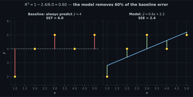
Worked example by hand

The Phase 3 five-point dataset with $\hat{y} = 0.6x + 2.2$ and $\bar{y} = 4$:

Step 1 — check the decomposition. $3.6 + 2.4 = 6.0$. It balances exactly, as it must.

Step 2 — compute $R^2$.

Step 3 — adjust for the one feature used. With $m = 5$ and $k = 1$:

The drop from 0.60 to 0.467 is the price of one feature on only five samples. On 5,000 samples the same feature would cost almost nothing — which is exactly the behaviour you want.

figureThe two sums of squares, side by sidematplotlib

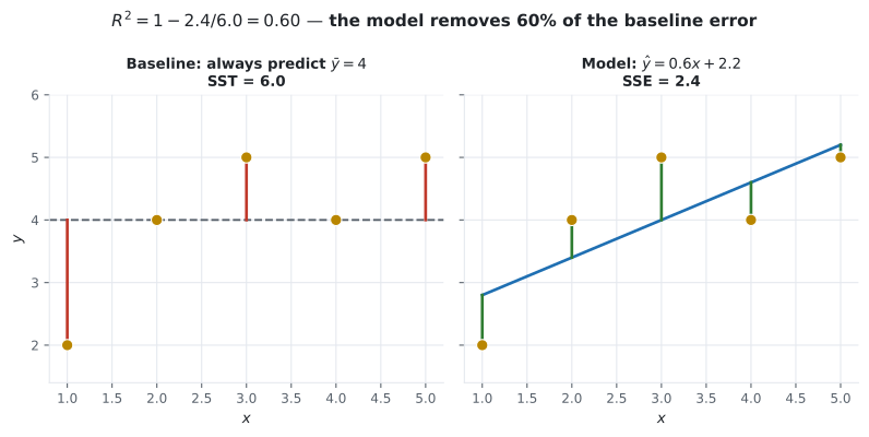
See it move

The animation sweeps from a flat mean-only baseline to the least-squares fit. Red stems are the baseline’s errors, green are the model’s — and $R^2$ tracks the ratio between them.

From scratch

import numpy as np
from sklearn.metrics import r2_score
 
 
def r_squared(y, pred):
    sse = float(((y - pred) ** 2).sum())
    sst = float(((y - y.mean()) ** 2).sum())
    return 1 - sse / sst
 
 
def adjusted_r_squared(y, pred, n_features):
    m = len(y)
    r2 = r_squared(y, pred)
    return 1 - (1 - r2) * (m - 1) / (m - n_features - 1)
 
 
x = np.array([1.0, 2.0, 3.0, 4.0, 5.0])
y = np.array([2.0, 4.0, 5.0, 4.0, 5.0])
pred = 0.6 * x + 2.2
 
sst = ((y - y.mean()) ** 2).sum()
ssr = ((pred - y.mean()) ** 2).sum()
sse = ((y - pred) ** 2).sum()
 
print(f"SST = {sst:.1f}")                 # SST = 6.0
print(f"SSR = {ssr:.1f}")                 # SSR = 3.6
print(f"SSE = {sse:.1f}")                 # SSE = 2.4
print(f"SSR + SSE = {ssr + sse:.1f}")     # SSR + SSE = 6.0
 
print(f"R^2      = {r_squared(y, pred):.4f}")               # R^2      = 0.6000
print(f"adjusted = {adjusted_r_squared(y, pred, 1):.4f}")   # adjusted = 0.4667
print(f"sklearn  = {r2_score(y, pred):.4f}")                # sklearn  = 0.6000

import numpy as np
from sklearn.metrics import r2_score
 
 
def r_squared(y, pred):
    sse = float(((y - pred) ** 2).sum())
    sst = float(((y - y.mean()) ** 2).sum())
    return 1 - sse / sst
 
 
def adjusted_r_squared(y, pred, n_features):
    m = len(y)
    r2 = r_squared(y, pred)
    return 1 - (1 - r2) * (m - 1) / (m - n_features - 1)
 
 
x = np.array([1.0, 2.0, 3.0, 4.0, 5.0])
y = np.array([2.0, 4.0, 5.0, 4.0, 5.0])
pred = 0.6 * x + 2.2
 
sst = ((y - y.mean()) ** 2).sum()
ssr = ((pred - y.mean()) ** 2).sum()
sse = ((y - pred) ** 2).sum()
 
print(f"SST = {sst:.1f}")                 # SST = 6.0
print(f"SSR = {ssr:.1f}")                 # SSR = 3.6
print(f"SSE = {sse:.1f}")                 # SSE = 2.4
print(f"SSR + SSE = {ssr + sse:.1f}")     # SSR + SSE = 6.0
 
print(f"R^2      = {r_squared(y, pred):.4f}")               # R^2      = 0.6000
print(f"adjusted = {adjusted_r_squared(y, pred, 1):.4f}")   # adjusted = 0.4667
print(f"sklearn  = {r2_score(y, pred):.4f}")                # sklearn  = 0.6000

Why $R^2$ alone is never enough

It rewards useless features

figureAdding columns of pure random noise to a two-feature problemmatplotlib

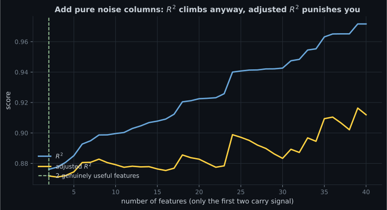
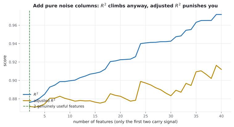
The mechanism is not subtle: with $m$ samples and $m-1$ features, a linear model can interpolate the training data exactly and score $R^2 = 1$ having learned nothing. Any model comparison across different feature counts must use adjusted $R^2$, cross-validation, or an information criterion.

It cannot see the shape of the data

figureAnscombe's quartet: four datasets, one set of statisticsmatplotlib

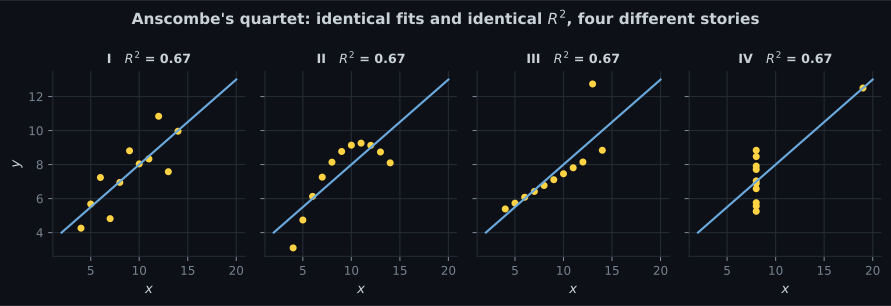
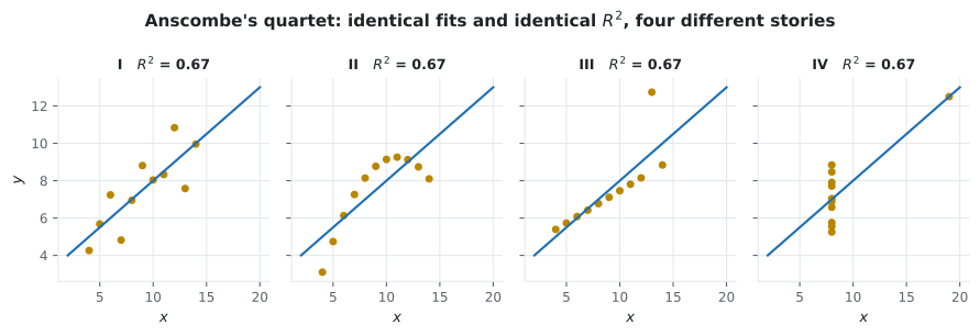
Reading the plots

• I is the only honest one — a genuine linear relationship with scatter.
• II is a perfect parabola. The linear model is systematically wrong everywhere, and $R^2$ cannot tell.
• III is a perfect straight line ruined by a single outlier, which drags the fit off the true relationship.
• IV has no relationship at all. Ten points share one $x$ value; a single leverage point at $x = 19$ determines the entire slope.

Constructed in 1973 to make exactly this argument, and the argument has not aged: plot your residuals. A metric is a summary, and summaries lose things.

Negative $R^2$ on real data

from sklearn.datasets import load_diabetes
from sklearn.linear_model import LinearRegression
from sklearn.model_selection import train_test_split
from sklearn.pipeline import make_pipeline
from sklearn.preprocessing import PolynomialFeatures
 
X, y = load_diabetes(return_X_y=True)
X_train, X_test, y_train, y_test = train_test_split(
    X, y, test_size=0.3, random_state=42
)
 
overfit = make_pipeline(
    PolynomialFeatures(4, include_bias=False),   # 10 features -> 1,000+
    LinearRegression(),
).fit(X_train, y_train)
 
print(f"train R^2 = {overfit.score(X_train, y_train):.4f}")   # train R^2 = 1.0000
print(f"test  R^2 = {overfit.score(X_test, y_test):.4f}")     # test  R^2 = -36.6836

from sklearn.datasets import load_diabetes
from sklearn.linear_model import LinearRegression
from sklearn.model_selection import train_test_split
from sklearn.pipeline import make_pipeline
from sklearn.preprocessing import PolynomialFeatures
 
X, y = load_diabetes(return_X_y=True)
X_train, X_test, y_train, y_test = train_test_split(
    X, y, test_size=0.3, random_state=42
)
 
overfit = make_pipeline(
    PolynomialFeatures(4, include_bias=False),   # 10 features -> 1,000+
    LinearRegression(),
).fit(X_train, y_train)
 
print(f"train R^2 = {overfit.score(X_train, y_train):.4f}")   # train R^2 = 1.0000
print(f"test  R^2 = {overfit.score(X_test, y_test):.4f}")     # test  R^2 = -36.6836

A perfect 1.0 on training and −36.68 on test. The model is thirty-seven times worse than a constant predictor on data it has not seen. Report only the training score and this looks like the best model ever built.

Which metric to report

Reasonable default: report RMSE and $R^2$ together, both on held-out data. RMSE gives the magnitude, $R^2$ gives the context, and neither is enough alone.

Pitfalls

🧪 Try It Yourself

Exercise 1 – Compute R-squared from two sums

Exercise 2 – Verify the decomposition

Exercise 3 – Adjust for the feature count

Exercise 4 – Watch noise inflate R-squared

Exercise 5 – Produce a negative R-squared

Recap

• $\text{SST} = \text{SSR} + \text{SSE}$ holds whenever the model has a least-squares intercept; $R^2 = 1 - \text{SSE}/\text{SST}$.
• On the five-point set: SST 6.0, SSR 3.6, SSE 2.4, so $R^2 = 0.60$ and adjusted $R^2 = 0.467$.
• $R^2$ compares against the mean baseline. Zero means no better than a constant; negative means worse, which happens routinely on held-out data.
• $R^2$ rises with every added feature, even pure noise. Use adjusted $R^2$ or cross-validation when feature counts differ.
• Anscombe’s quartet: four datasets, one fitted line, one $R^2$, four different truths.
• Report RMSE and $R^2$ together, always on held-out data, and always look at the residual plot.

Exercise 6 – Buy $R^2$ with pure noise

Next

Phase 3 ends here. Continue to Phase 4 - Supervised Learning - Classification — the same machinery pointed at a target that takes labels instead of numbers, where a whole new family of metrics becomes necessary.